Color Interpolation
Interpolation is a type of estimation that finds new data points based on the range of a discrete set of known data points. When used in the context of color, it is finding one or more colors that reside between any two given colors. This is often used to simulate mixing colors, creating gradients, or even create color palettes.
ColorAide provides a number of useful utilities based on interpolation.
Linear Interpolation
Linear interpolation is registered in Color by Default
One of the most common, and easiest, ways to interpolate data between two points is to use linear interpolation. An easy way of thinking about this concept is to imagine drawing a straight line that connects two colors within a color space. We could then navigate along that line and return colors at different points to simulate mixing colors at various percentages or return the whole range and create a continuous, smooth gradient.
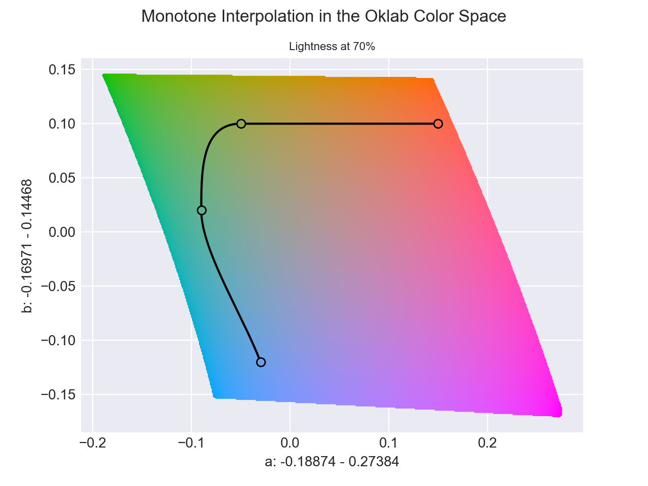
To further illustrate this point, the example below shows a slice of the Oklab color space at a lightness of 70%. On
this 2D plane, we select two colors: oklab(0.7 0.15 0.1) and oklab(0.7 -0.03 -0.12). We then connect
these two colors with a line. We can then select any point on the line to simulate the mixing of these colors. 0% would
yield the first color, 100% would yield the second color, and 50% would yield a new color:
oklab(0.7 0.06 -0.01).
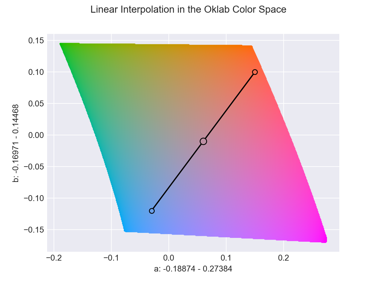
Figure 1. Interpolation performed at 50%
The interpolate method allows a user to create a linear interpolation function using two or more colors. By default, a
returned interpolation function accepts numerical input in the domain of [0, 1] and will cause a new color
between the specified colors to be returned.
By default, colors are interpolated in the perceptually uniform Oklab color space, though any supported color space can
be used instead. This also applies to all methods that use interpolation, such as discrete,
steps, mix, etc.
As an example, below we create an interpolation between rebeccapurple and lch(85% 100 85). We then
step through values of 0.0, 0.1, 0.2, etc. This returns colors at various positions on the line that connects
the two colors, 0 returning rebeccapurple and 1 returning lch(85% 100 85).
>>> i = Color.interpolate(["rebeccapurple", "lch(85% 60 85)"], space='lch')
>>> [i(x / 10).to_string() for x in range(10 + 1)]
['lch(32.393 61.244 308.86)', 'lch(37.653 61.119 322.47)', 'lch(42.914 60.995 336.09)', 'lch(48.175 60.87 349.7)', 'lch(53.436 60.746 3.3143)', 'lch(58.696 60.622 16.929)', 'lch(63.957 60.497 30.543)', 'lch(69.218 60.373 44.157)', 'lch(74.479 60.249 57.771)', 'lch(79.739 60.124 71.386)', 'lch(85 60 85)']
If we create enough steps, we can create a gradient.
Piecewise Interpolation
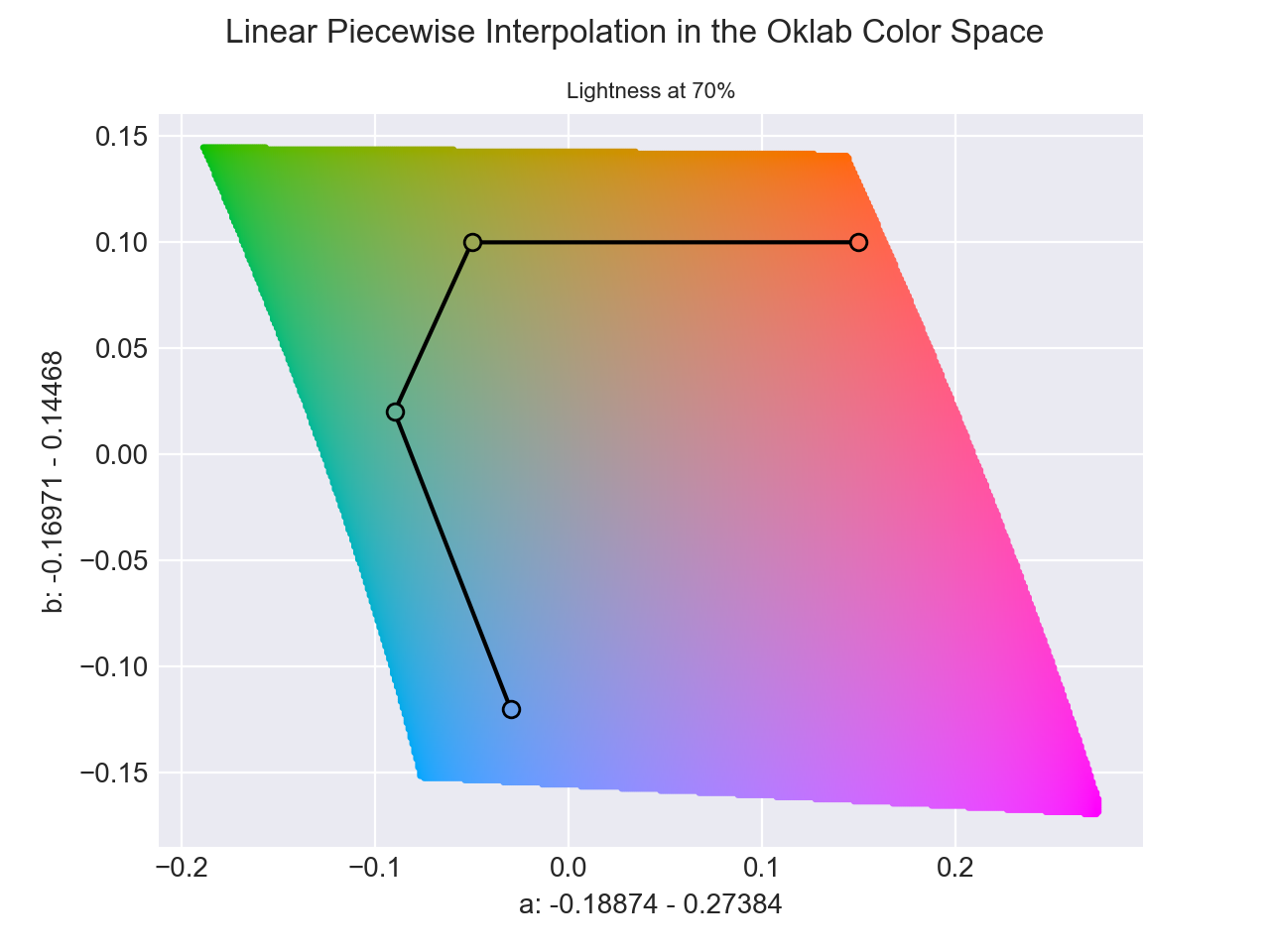
Piecewise interpolation takes the idea of linear interpolation and then applies it to multiple colors. As drawing a straight line through a series of points greater than two can be difficult to achieve, piecewise interpolation creates straight lines between each color in a chain of colors.
When the interpolate method receives more that two colors, the interpolation will utilize piecewise interpolation
and interpolation will be broken up between each pair of colors. The function, just like when interpolating between two
colors, still operates by default in the domain of [0, 1], only it will now apply to the entire range of colors.
Piecewise interpolation simply breaks up a series of data points into segments in order to apply interpolation individually on each segment.
This approach generally works well, but since the placement of colors may not be in a straight line, you will often have pivot points and the transition may not be quite as smooth at these locations.
Continuous Interpolation
Continuous interpolation is registered in Color by Default
In this document, we use the term "continuous" in two ways when talking about interpolation: continuous vs
discrete and the interpolation method whose literal name is continuous.
The continuous interpolation approach, is simply a piecewise, linear interpolation method that interpolates defined
channels continuously across two or more segments with undefined channels, essentially taking into account all the
segments in the piecewise chain when processing undefined channels. This differs from the default CSS piecewise
interpolation approach which only takes into context two segments at any given time. What this means is that if you have
multiple colors, and one or more of the colors have the same channel undefined, the colors with that channel defined
will be interpolated across the undefined gaps spanning one or more segments in the chain.
In this example, we have 3 colors. The end colors both define lightness, but the middle color is undefined. We can see
that when we use normal, linear piecewise interpolation that we get a discontinuity. But with continuous
interpolation, we get a smooth interpolation of the lightness through the undefined channel.
>>> colors = [
...     Color('oklab', [0, 0, 0]),
...     Color('oklab', [NaN, -0.03246, -0.31153]),
...     Color('oklab', [1, 0, 0])
... ]
>>> Color.interpolate(colors, space='oklab', method='linear')
<coloraide.interpolate.linear.InterpolatorLinear object at 0x7fc17c757100>
>>> Color.interpolate(colors, space='oklab', method='continuous')
<coloraide.interpolate.continuous.InterpolatorContinuous object at 0x7fc17d3ab380>
Now, if we have colors on the side that are not between two defined colors, all those colors will adopt the defined
value of the first color on either the right or left that is defined. In the example below, we have a single color with
all components defined, but all the colors to the left are missing the lightness. Again, in the normal linear
approach, we see a discontinuity, but with the continous approach, all colors with the undefined lightness will assume
the lightness of the defined color.
>>> colors = [
...     Color('oklab', [NaN, 0.22486, 0.12585]),
...     Color('oklab', [NaN, -0.1403, 0.10768]),
...     Color('oklab', [0.45201, -0.03246, -0.31153])
... ]
>>> Color.interpolate(colors, space='oklab', method='linear')
<coloraide.interpolate.linear.InterpolatorLinear object at 0x7fc17c757100>
>>> Color.interpolate(colors, space='oklab', method='continuous')
<coloraide.interpolate.continuous.InterpolatorContinuous object at 0x7fc17c781a90>
This approach is useful for more natural, multi-color interpolations and is used as foundation for our spline interpolation approaches which often require the context of at least four colors when applying their logic.
Spectral
New in 8.8
Spectral interpolation is not registered in Color by Default
>>> from coloraide import Color
>>> from coloraide.interpolate.spectral import Spectral
>>> class Custom(Color): ...
...
>>> Custom.register(Spectral())
>>> Custom.interpolate(['#51A5E6', '#79AF58', '#92A854', '#A097BE', '#CF8E38', '#CF83A1', '#F76B5C'], method='spectral')
<coloraide.interpolate.spectral.InterpolatorSpectralLinear object at 0x7fc17d3ab380>
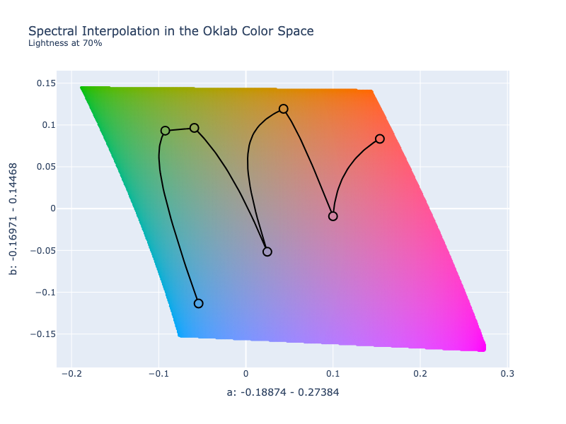
Spectral interpolation attempts to mix colors similar to how they are done in paint using Kubelka-Munk theory.
>>> red = Color('rgb(128, 2, 46)').mix('white', 0.25, method='spectral')
>>> yellow = Color('rgb(252, 211, 0)').mix('white', 0.25, method='spectral')
>>> blue = Color('rgb(13, 27, 68)').mix('white', 0.25, method='spectral')
>>> Wheel(Color.steps([red, yellow, blue, red], steps=13, method='spectral', out_space='srgb')[:-1])
[color(srgb 0.68578 0.08554 0.31995 / 1), color(srgb 0.75582 0.16989 0.25944 / 1), color(srgb 0.89803 0.36103 0.22514 / 1), color(srgb 0.9821 0.63606 0.18224 / 1), color(srgb 0.98893 0.84036 0.07637 / 1), color(srgb 0.78301 0.80074 0.1552 / 1), color(srgb 0.49196 0.65013 0.24437 / 1), color(srgb 0.24597 0.44964 0.34055 / 1), color(srgb 0.20994 0.33965 0.59238 / 1), color(srgb 0.26453 0.26232 0.53216 / 1), color(srgb 0.35077 0.16742 0.40469 / 1), color(srgb 0.53163 0.12631 0.33717 / 1)]
>>> Steps(Color.steps([red, yellow, blue, red], steps=13, method='spectral', out_space='srgb')[:-1])
[color(srgb 0.68578 0.08554 0.31995 / 1), color(srgb 0.75582 0.16989 0.25944 / 1), color(srgb 0.89803 0.36103 0.22514 / 1), color(srgb 0.9821 0.63606 0.18224 / 1), color(srgb 0.98893 0.84036 0.07637 / 1), color(srgb 0.78301 0.80074 0.1552 / 1), color(srgb 0.49196 0.65013 0.24437 / 1), color(srgb 0.24597 0.44964 0.34055 / 1), color(srgb 0.20994 0.33965 0.59238 / 1), color(srgb 0.26453 0.26232 0.53216 / 1), color(srgb 0.35077 0.16742 0.40469 / 1), color(srgb 0.53163 0.12631 0.33717 / 1)]
Tip
Unlike other interpolation methods, the default interpolation space is treated as XYZ D65 instead of Oklab. This is
true regardless of what the default for the Color object is. If a space is explicitly defined, the color will be
output in that space (unless output_space overrides it), but the color will still be processed in XYZ D65.
Light, on its own, doesn't mix like pigments due to the way pigments absorb and scatter light. Kubelka-Munk theory is a fundamental approach to modelling the appearance of paint films and predicting this absorption and scattering. Utilizing Kubelka-Munk theory, colors can be simulated to mix more like paints.
>>> c1 = Color('#002185')
>>> c2 = Color('#FCD200')
>>> Color.interpolate([c1, c2], method='spectral')
<coloraide.interpolate.spectral.InterpolatorSpectralLinear object at 0x7fc17c795ae0>
>>> Steps(Color.steps([c1, c2], method='spectral', steps=9))
[color(xyz-d65 0.04777 0.02781 0.22476 / 1), color(xyz-d65 0.02667 0.03298 0.0951 / 1), color(xyz-d65 0.03708 0.06387 0.07248 / 1), color(xyz-d65 0.07117 0.12699 0.07519 / 1), color(xyz-d65 0.13265 0.22305 0.08176 / 1), color(xyz-d65 0.22548 0.34363 0.08795 / 1), color(xyz-d65 0.34991 0.47284 0.09246 / 1), color(xyz-d65 0.49784 0.59012 0.09493 / 1), color(xyz-d65 0.6319 0.6679 0.09564 / 1)]
>>> c1 = Color('#002185')
>>> c2 = Color('#FCD200')
>>> Color.interpolate([c1, c2], space='srgb')
<coloraide.interpolate.linear.InterpolatorLinear object at 0x7fc17c30d250>
>>> Steps(Color.steps([c1, c2], space='srgb', steps=9))
[color(srgb 0 0.12941 0.52157 / 1), color(srgb 0.12353 0.21618 0.45637 / 1), color(srgb 0.24706 0.30294 0.39118 / 1), color(srgb 0.37059 0.38971 0.32598 / 1), color(srgb 0.49412 0.47647 0.26078 / 1), color(srgb 0.61765 0.56324 0.19559 / 1), color(srgb 0.74118 0.65 0.13039 / 1), color(srgb 0.86471 0.73676 0.0652 / 1), color(srgb 0.98824 0.82353 0 / 1)]
It is important to note that actual paint mixing is more complicated than what we do here in ColorAide. Every paint has its own specific properties related to the absorption and scattering of light due to the properties of the paint particles. Since we are not basing our approach off real paint data, we do not have these specific constants and opt for a simplified, single-constant approach when applying Kubelka-Munk theory, opposed to the more accurate two-constant approach.
Paint-like mixing, as is implemented here, is a more simplified approach that approximates the look and feel of paint mixing in general. This is based on the work of Scott Burns who developed a way to approximate reflectance curves from sRGB triplets. The project Spectral.js ran with this idea and applied Kubelka-Munk theory to transform these reflectance curves into scattering/absorption coefficients so that the curves could be mixed linearly, producing paint like mixing. ColorAide adopts this same approach with minor modifications.
In principle, if we were to approximate the reflectance curves of rgb(255 0 0), rgb(0 255 0 ), and
rgb(0 0 255), using the approach by Scott Burns, such that they also summed up to 1, we could likely calculate
reflectance curves from these three colors and approximate reflectance curves for almost any other color in the sRGB
gamut. Unfortunately, this creates a non-linearity problem that is difficult to solve with high precision, so instead,
we calculate primary reflectance curves from 7 colors individually so that, when combined, we can generate smooth
approximations for almost any color within the sRGB gamut.
| Primary Reflectance Curves |
|---|
rgb(255 0 0) |
rgb(0 255 0) |
rgb(0 0 255) |
rgb(0 255 255) |
rgb(255 0 255) |
rgb(255 255 0) |
rgb(255 255 255) |
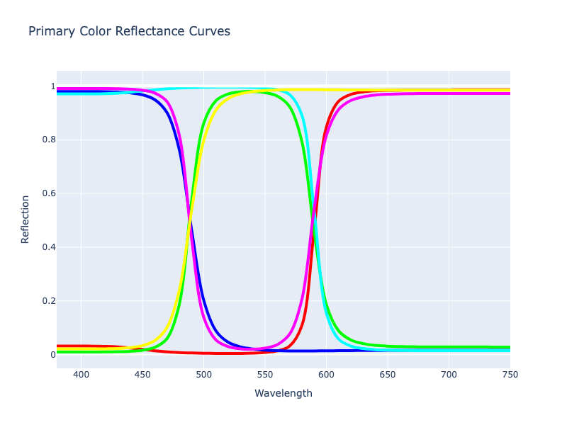
Figure 2. Reflectance curves of white, cyan, magenta, yellow, red, green, and blue as approximated using the methods proposed by Scott Burns.
With our primary colors selected, and the reflectance curves created for each one, we can use these curves to approximate smooth reflectance curves for almost any color within the sRGB gamut by deconstructing a given color into concentrations of these primary reflectance curves and then combining them into a new curve that represents the color.
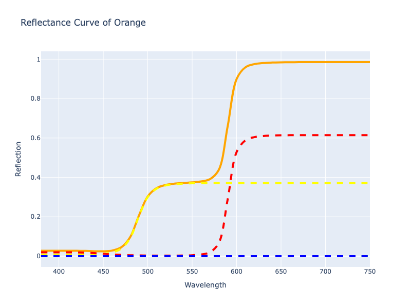
Figure 3. Orange decomposed into white, cyan, magenta, yellow, red, green, and blue reflectance curves and then reconstructed into its own curve.
With the ability to represent almost any color within our gamut as a reflectance curve, we then can mix colors by generating their curve and then applying Kubelka-Munk theory by converting those curves into absorption and scattering coefficients and mixing them linearly. Once mixed, we can transform them back to a reflectance curve and then back to our target color space.
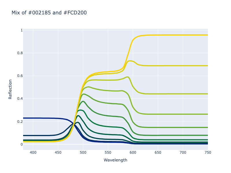
Figure 4. Mixing a blue and yellow color with Kubelka-Munk theory.
It should be noted that when using this approach, the mixing of the colors can turn out a bit dark. The author of Spectral.js noticed this and found that weighting the mix such that more luminous colors had more weight produced more natural lighting when mixing.
One way that ColorAide deviates from the Spectral.js is that we ensure sane behavior for colors that extend beyond the sRGB gamut. Using the approach as described works for most colors within the sRGB gamut, but doesn't precisely cover every color perfectly, and will be less usable for colors outside the sRGB gamut. This is because Kubelka-Munk does not handle reflectance values above 1 well. Certain combinations of reflectance curves will produce reflectance values that exceed 1.
Borrowing an idea from the paper released by the creators of Mixbox, ColorAide goes further and first ensures a given approximated color curve does not exceed a reflectance of 1 at any point within the curve. Then we calculate the residual XYZ values between the original color and what our limited reflectance curve can produce. The residuals of the colors being mixed are interpolated directly within the XYZ space and added back into the final result once the reflectance curves have been mixed. This allows for sane handling for wider gamut colors.
>>> c1 = Color('color(display-p3 0 0 1)')
>>> c2 = Color('color(display-p3 1 1 0)')
>>> Color.interpolate([c1, c2], method='spectral')
<coloraide.interpolate.spectral.InterpolatorSpectralLinear object at 0x7fc17c771c50>
>>> Steps(Color.steps([c1, c2], method='spectral', steps=9))
[color(xyz-d65 0.19822 0.07929 1.0439 / 1), color(xyz-d65 0.06051 0.0615 0.29103 / 1), color(xyz-d65 0.05131 0.07666 0.17683 / 1), color(xyz-d65 0.07157 0.12065 0.13913 / 1), color(xyz-d65 0.12297 0.20065 0.11708 / 1), color(xyz-d65 0.21721 0.32545 0.09921 / 1), color(xyz-d65 0.36095 0.49724 0.08216 / 1), color(xyz-d65 0.54818 0.70664 0.06461 / 1), color(xyz-d65 0.75224 0.92071 0.04511 / 1)]
Spectral mixing comes in too flavors: normal and continuous.
>>> colors = [
...     Color('#00000000'),
...     Color('#002185').set('alpha', NaN),
...     Color('#FFFFFFFF')
... ]
>>> Color.interpolate(colors, method='spectral')
<coloraide.interpolate.spectral.InterpolatorSpectralLinear object at 0x7fc17c771d50>
>>> Color.interpolate(colors, method='spectral-continuous')
<coloraide.interpolate.spectral.InterpolatorSpectralContinuous object at 0x7fc17d3ab380>
To enable spectral-continuous, simply register it like you would spectral.
>>> from coloraide import Color
>>> from coloraide.interpolate.spectral import SpectralContinuous
>>> class Custom(Color): ...
...
>>> Custom.register(SpectralContinuous())
>>> Custom.interpolate(['#51A5E6', '#79AF58', '#92A854', '#A097BE', '#CF8E38', '#CF83A1', '#F76B5C'], method='spectral-continuous')
<coloraide.interpolate.spectral.InterpolatorSpectralContinuous object at 0x7fc17c7811d0>
Cubic Spline Interpolation
Linear interpolation is nice because it is easy to implement, and due to its straight forward nature, pretty fast. With that said, it doesn't always have the smoothest transitions. It turns out that there are other piecewise ways to interpolate that can yield smoother results.
Inspired by some efforts seen on the web and in the great JavaScript library Culori, ColorAide implements a number of spline based interpolation methods.
Because splines require taking into account more than two colors at a time, all spline based interpolation methods are
built off of the continuous interpolation approach of handling undefined values.
B-Spline
B-Spline interpolation is registered in Color by Default
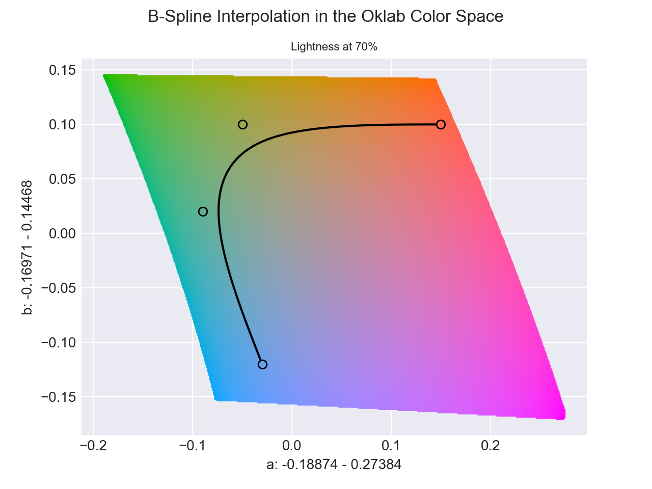
B-spline is a piecewise spline similar to Bezier curves. It utilizes "control points" that help shape the interpolation path through a series of colors. Like Bezier Curves, the path is not guaranteed to pass through the control points.
Tip
By default, this approach uses not-a-knot end conditions which doesn't introduce end point bias, but if you'd like to
ensure the interpolation passes through the end points, you can set end_cond to natural.
If you need an interpolation to pass through all points, see the Natural spline.
Natural
Natural interpolation is registered in Color by Default
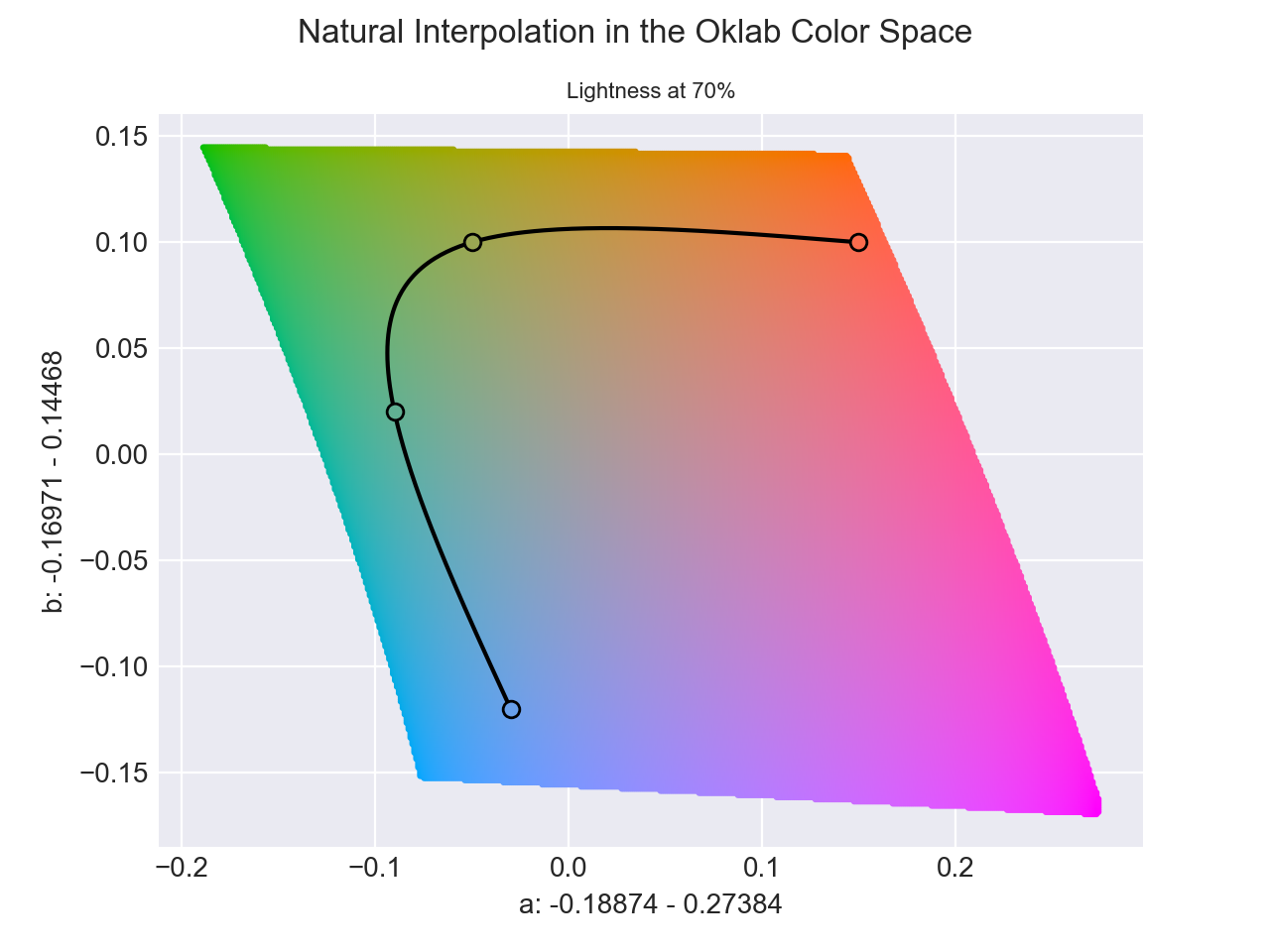
The "natural" spline is the same as the B-spline approach except an algorithm is applied that uses the colors as data points and calculates new control points such that the interpolation passes through all the data points. This means that the path will pass through all the colors. The resultant spline has the continuity and properties of a natural spline, hence the name.
- Interpolation: Passes through all control points.
- Continuity: C2 continuous (both first and second derivatives are continuous).
- Local control: No, changing one point affects the entire curve.
- Boundary Conditions: Uses "natural" conditions (second derivative = 0 at endpoints).
Natural provides a nice, smooth curve, but may have unwanted oscillations. Occasionally it can cause the interpolation path to pass out of gamut if interpolating on an edge.
It can be used by specifying natural as the interpolation method.
Tip
By default, end conditions are set to natural, and while not recommended, you can set end_cond to not-a-not, but
that would undo the behavior that constrains the interpolation to pass through the end points, a characteristic of the
natural boundary conditions.
Catmull-Rom
Catmull-Rom interpolation is not registered in Color by Default

>>> from coloraide import Color
>>> from coloraide.interpolate.catmull_rom import CatmullRom
>>> class Custom(Color): ...
...
>>> Custom.register(CatmullRom())
>>> Custom.interpolate(['#51A5E6', '#79AF58', '#92A854', '#A097BE', '#CF8E38', '#CF83A1', '#F76B5C'], method='catrom')
<coloraide.interpolate.catmull_rom.InterpolatorCatmullRom object at 0x7fc17d3aacf0>
The Catmull-Rom spline is another "interpolating" spline that passes through all of its data points, similar to the "natural" spline in that it passes through all the points, but it but does not share the same continuity and properties of a "natural" spline.
- Interpolation: Passes through all control points.
- Continuity: C1 continuous (first derivative is continuous).
- Local Control: Adjustments of one point won't affect the entire curve.
With Catmull-Rom, changing one point won't affect the entire curve, but has a more local effect. Depending on the data set, can have more overshoot than Natural and can exhibit unwanted oscillation.
Tip
By default, catrom uses not-a-knot end conditions which do not introduce end point bias, but you can set
end_cond to natural if preferred which will guide the interpolation through the end points in a more linear way at
the ends.
Monotone
Monotone interpolation is registered in Color by Default
The "monotone" spline is a piecewise interpolation spline that passes through all its data points and helps to preserve monotonicity. As far as we are concerned, the important thing to note is that it greatly reduces any overshoot or undershoot in the interpolation.
- Interpolation: Passes through all control points.
- Continuity: C1 continuous (first derivative continuous).
- Local control: Adjustments of one point won't affect the entire curve.
Much like Catmull-Rom, adjusting one point won't affect the entire curve, but it ensures the interpolated curve maintains the increasing or decreasing trend. As previously mentioned, this also prevents oscillations, but can sometimes be too constrained and give less smooth results.
Tip
By default, monotone uses not-a-knot end conditions which do not introduce end point bias, but you can set
end_cond to natural if preferred which will guide the interpolation through the end points in a more linear way at
the ends.
Discrete Interpolation
So far, we've only shown examples of continuous interpolation methods. To clarify, we are using "continuous" in a
slightly different way than we discussed earlier. When we say "continuous" here, we simply
mean that the colors in the interpolation smoothly transition from one color to the other. But when creating charts or
graphs, some times you'd like to categorize data such that a range of values correspond to a specific color. For this,
we can use discrete, which like intrpolate, returns an interpolation object, but the ranges will be discrete.
By default, ranges are calculated directly form the input colors. So if you had three colors, the interpolation would be broken up into 3 ranges. Compare this with the "continuous" interpolation we methods we showed earlier.
If we specify step, we can create a larger or smaller color scale using the input colors to interpolate the new color
scale. And we can use any of the aforementioned interpolation methods to help generate this new discrete scale.
What makes this really useful is if you combine it with custom domains to process data. By default, the domain is
[0, 1], but we can change this to directly correlate the data with our quantized color samples. For instance, let's
use a series of discrete colors to represent temperature. Additionally, let's use domain to associate a
temperature ranges with the given colors. Now when we input a temperature value, it will align with our discrete color
scale.
>>> i = Color.discrete(['blue', 'green', 'yellow', 'orange', 'red'], domain=[-32, 32, 60, 85, 95])
>>> i(-32)
color(--oklab 0.45201 -0.03246 -0.31153 / 1)
>>> i(40)
color(--oklab 0.51975 -0.1403 0.10768 / 1)
>>> i(87)
color(--oklab 0.79269 0.05661 0.16138 / 1)
>>> i(100)
color(--oklab 0.62796 0.22486 0.12585 / 1)
>>> i
<coloraide.interpolate.linear.InterpolatorLinear object at 0x7fc17c771350>
Additionally, color scales can be limited using the padding parameter.
As discrete() is built on steps(), it can take all the same arguments. Check out steps() to
learn more.
Hue Interpolation
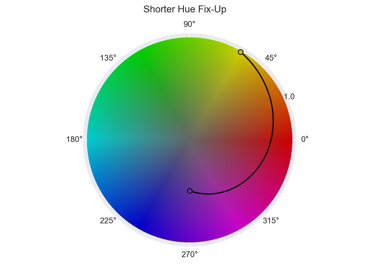
In interpolation, hues are handled special allowing us to control the way in which hues are evaluated. By default, the
shortest angle between two hues is targeted for interpolation, but the hue option allows us to redefine this behavior
in a number of interesting ways: shorter, longer, increasing, decreasing, and specified. These hue "fix-ups"
identify all possible ways in which we can interpolate a hue and come from the
CSS level 4 specification.
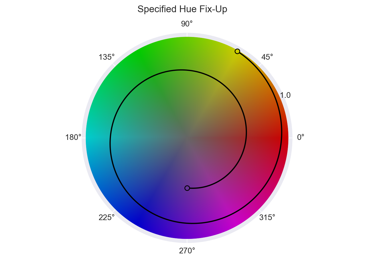
Specified
The specified fix-up was at one time specified in the CSS Color Level 4 specification, but is no longer mentioned
there. While CSS no longer supports this hue fix-up, we still do. specified simply does not apply any hue fix-up and
will use hues as specified, hence the name.
To help visualize the different hue methods, consider the following evaluation between hsl(270 50 40) and
hsl(780 100 40). Below we will demonstrate each of the different hue evaluations and explain what it is that
they do.
shorter interpolates along the shortest arc length after normalizing the hues.
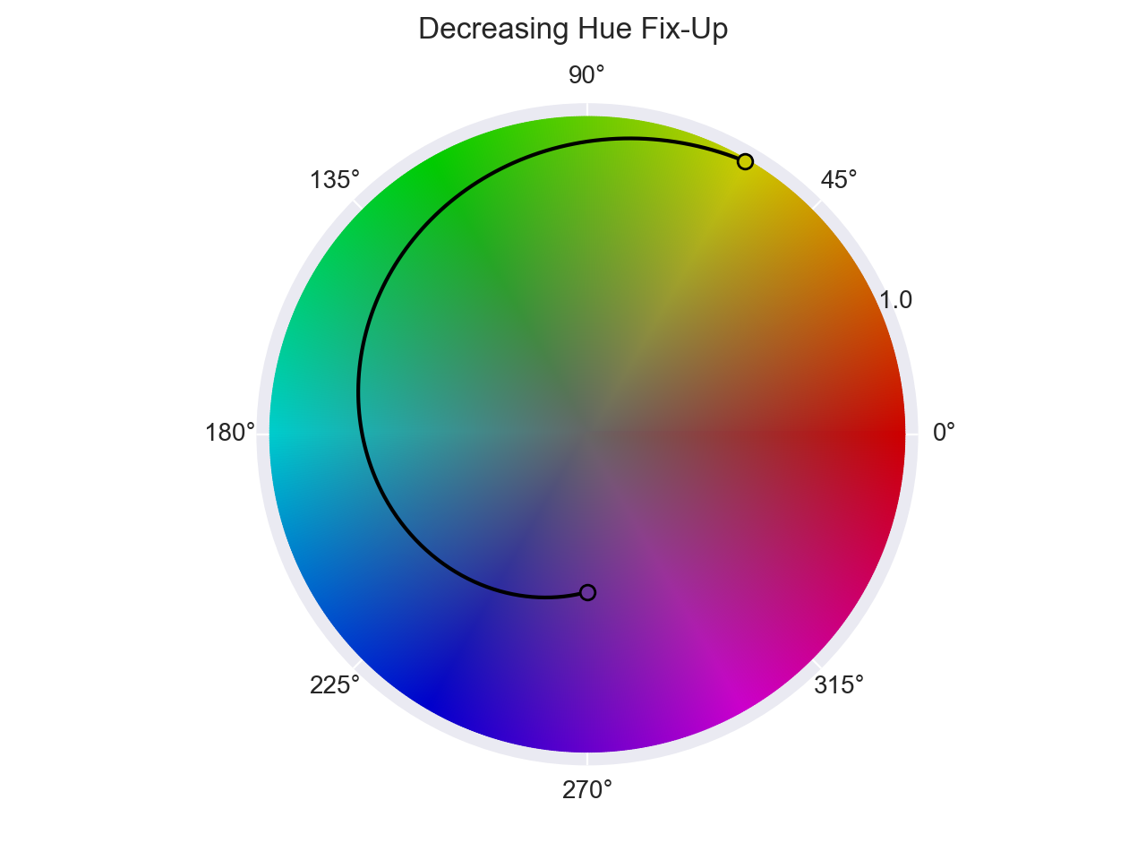
longer interpolates along the longest arc length after normalizing the hues.

increasing interpolates counter clockwise (after normalizing the hues), such that the hues are increasing.

decreasing interpolates clockwise (after normalizing the hues), such that the hues are decreasing.
Interpolating with Alpha
Interpolating color channels is pretty straight forward and uses traditional linear interpolation logic, but when introducing transparency to a color, interpolation uses a concept known as premultiplication which alters the normal interpolation process.
Premultiplication is a technique that tends to produce better results when two colors have differing transparency. It essentially accounts for the transparency and uses it to weight how may a given color channel will contribute to the interpolation. A more transparent color's channels will naturally contribute less.
Consider the following example. Normally, when transitioning to a "transparent" color, the colors will be more gray
during the transition. This is because transparent is actually black. But when using premultiplication, the
transition looks just as one would expect as the transparent color's channels are weighted less due to the high
transparency.
As a final example, below we have an opaque orange and a blue that is quite transparent. Logically, the blue shouldn't have as big an affect on the overall color as it is so faint, and yet, in the un-premultiplied example, when mixing the colors equally, we see that the resultant color is also equally influenced by the hue of both colors. In the premultiplied example, we see that orange is still quite dominant at 50% as it is fully opaque.
If we interpolate it, we can see the difference in transition.
>>> Color.interpolate(['orange', Color('blue').set('alpha', 0.25)], space='srgb', premultiplied=False)
<coloraide.interpolate.linear.InterpolatorLinear object at 0x7fc17c771450>
>>> Color.interpolate(['orange', Color('blue').set('alpha', 0.25)], space='srgb')
<coloraide.interpolate.linear.InterpolatorLinear object at 0x7fc17c771d50>
There may be some cases where it is desired to use no premultiplication in alpha blending. One could simply be that you
need to mimic the same behavior of a system that does not use premultiplied interpolation. If so, simply set
premultiplied to False as shown above.
Mixing
Interpolation Options
Any options not consumed by mix will be passed to the underlying interpolation function. This includes options
like hue, progress, etc.
The mix function is built on top of the interpolate function and provides a simple, quick,
and intuitive simple mixing of two colors. Just pass in a color to mix with the base color, and you'll get an equal mix
of the two.
By default, colors are mixed at 50%, but the percentage can be controlled. Here we mix the color blue into
the color red at 20%. With blue at 20% and red at 80%, this gives us a more reddish color.
As with all interpolation based functions, if needed, a different color space can be specified with the space
parameter or even a different interpolation method via method. mix accepts all the same parameters used in
interpolate, though concepts like stops and hints are not allowed with mixing.
Mix can also accept a string and will create the color for us which is great if we don't need to work with the second color afterwards.
Mixing will always return a new color unless in_place is set True.
Weighted Mixing
New in 8.8
While mix provides a way to mix any two colors together, weighted_mix allows the mixing of any number of
colors.
Instead of using a single percentage to indicate what color on an interpolation line you desire, weighted_mix takes a
list of weights that allows you to specify ratios of colors.
Below, we are going to mix 3 parts orange to 2 parts purple to 1 part white within Oklab.
By changing the weights, we can change the color.
>>> from coloraide import algebra as alg
>>> Steps(
...     [Color.weighted_mix(['orange', 'purple', 'white'], [3, i, j])
...     for i, j in zip(alg.linspace(0, 10, 100), alg.linspace(10, 0, 100))]
... )
[color(--oklab 0.95216 0.01306 0.03724 / 1), color(--oklab 0.94766 0.01434 0.03645 / 1), color(--oklab 0.94316 0.01562 0.03567 / 1), color(--oklab 0.93866 0.0169 0.03488 / 1), color(--oklab 0.93416 0.01818 0.03409 / 1), color(--oklab 0.92966 0.01946 0.0333 / 1), color(--oklab 0.92516 0.02074 0.03251 / 1), color(--oklab 0.92066 0.02202 0.03172 / 1), color(--oklab 0.91616 0.0233 0.03094 / 1), color(--oklab 0.91166 0.02458 0.03015 / 1), color(--oklab 0.90716 0.02586 0.02936 / 1), color(--oklab 0.90266 0.02714 0.02857 / 1), color(--oklab 0.89816 0.02842 0.02778 / 1), color(--oklab 0.89367 0.0297 0.02699 / 1), color(--oklab 0.88917 0.03098 0.0262 / 1), color(--oklab 0.88467 0.03226 0.02542 / 1), color(--oklab 0.88017 0.03354 0.02463 / 1), color(--oklab 0.87567 0.03482 0.02384 / 1), color(--oklab 0.87117 0.0361 0.02305 / 1), color(--oklab 0.86667 0.03738 0.02226 / 1), color(--oklab 0.86217 0.03866 0.02147 / 1), color(--oklab 0.85767 0.03994 0.02069 / 1), color(--oklab 0.85317 0.04122 0.0199 / 1), color(--oklab 0.84867 0.0425 0.01911 / 1), color(--oklab 0.84417 0.04378 0.01832 / 1), color(--oklab 0.83967 0.04506 0.01753 / 1), color(--oklab 0.83517 0.04634 0.01674 / 1), color(--oklab 0.83067 0.04762 0.01595 / 1), color(--oklab 0.82617 0.0489 0.01517 / 1), color(--oklab 0.82167 0.05018 0.01438 / 1), color(--oklab 0.81717 0.05146 0.01359 / 1), color(--oklab 0.81267 0.05274 0.0128 / 1), color(--oklab 0.80817 0.05402 0.01201 / 1), color(--oklab 0.80368 0.0553 0.01122 / 1), color(--oklab 0.79918 0.05658 0.01044 / 1), color(--oklab 0.79468 0.05786 0.00965 / 1), color(--oklab 0.79018 0.05914 0.00886 / 1), color(--oklab 0.78568 0.06042 0.00807 / 1), color(--oklab 0.78118 0.06169 0.00728 / 1), color(--oklab 0.77668 0.06297 0.00649 / 1), color(--oklab 0.77218 0.06425 0.00571 / 1), color(--oklab 0.76768 0.06553 0.00492 / 1), color(--oklab 0.76318 0.06681 0.00413 / 1), color(--oklab 0.75868 0.06809 0.00334 / 1), color(--oklab 0.75418 0.06937 0.00255 / 1), color(--oklab 0.74968 0.07065 0.00176 / 1), color(--oklab 0.74518 0.07193 0.00097 / 1), color(--oklab 0.74068 0.07321 0.00019 / 1), color(--oklab 0.73618 0.07449 -0.0006 / 1), color(--oklab 0.73168 0.07577 -0.00139 / 1), color(--oklab 0.72718 0.07705 -0.00218 / 1), color(--oklab 0.72268 0.07833 -0.00297 / 1), color(--oklab 0.71818 0.07961 -0.00376 / 1), color(--oklab 0.71369 0.08089 -0.00454 / 1), color(--oklab 0.70919 0.08217 -0.00533 / 1), color(--oklab 0.70469 0.08345 -0.00612 / 1), color(--oklab 0.70019 0.08473 -0.00691 / 1), color(--oklab 0.69569 0.08601 -0.0077 / 1), color(--oklab 0.69119 0.08729 -0.00849 / 1), color(--oklab 0.68669 0.08857 -0.00928 / 1), color(--oklab 0.68219 0.08985 -0.01006 / 1), color(--oklab 0.67769 0.09113 -0.01085 / 1), color(--oklab 0.67319 0.09241 -0.01164 / 1), color(--oklab 0.66869 0.09369 -0.01243 / 1), color(--oklab 0.66419 0.09497 -0.01322 / 1), color(--oklab 0.65969 0.09625 -0.01401 / 1), color(--oklab 0.65519 0.09753 -0.01479 / 1), color(--oklab 0.65069 0.09881 -0.01558 / 1), color(--oklab 0.64619 0.10009 -0.01637 / 1), color(--oklab 0.64169 0.10137 -0.01716 / 1), color(--oklab 0.63719 0.10265 -0.01795 / 1), color(--oklab 0.63269 0.10393 -0.01874 / 1), color(--oklab 0.62819 0.10521 -0.01952 / 1), color(--oklab 0.62369 0.10649 -0.02031 / 1), color(--oklab 0.6192 0.10777 -0.0211 / 1), color(--oklab 0.6147 0.10905 -0.02189 / 1), color(--oklab 0.6102 0.11033 -0.02268 / 1), color(--oklab 0.6057 0.11161 -0.02347 / 1), color(--oklab 0.6012 0.11288 -0.02426 / 1), color(--oklab 0.5967 0.11416 -0.02504 / 1), color(--oklab 0.5922 0.11544 -0.02583 / 1), color(--oklab 0.5877 0.11672 -0.02662 / 1), color(--oklab 0.5832 0.118 -0.02741 / 1), color(--oklab 0.5787 0.11928 -0.0282 / 1), color(--oklab 0.5742 0.12056 -0.02899 / 1), color(--oklab 0.5697 0.12184 -0.02977 / 1), color(--oklab 0.5652 0.12312 -0.03056 / 1), color(--oklab 0.5607 0.1244 -0.03135 / 1), color(--oklab 0.5562 0.12568 -0.03214 / 1), color(--oklab 0.5517 0.12696 -0.03293 / 1), color(--oklab 0.5472 0.12824 -0.03372 / 1), color(--oklab 0.5427 0.12952 -0.03451 / 1), color(--oklab 0.5382 0.1308 -0.03529 / 1), color(--oklab 0.5337 0.13208 -0.03608 / 1), color(--oklab 0.52921 0.13336 -0.03687 / 1), color(--oklab 0.52471 0.13464 -0.03766 / 1), color(--oklab 0.52021 0.13592 -0.03845 / 1), color(--oklab 0.51571 0.1372 -0.03924 / 1), color(--oklab 0.51121 0.13848 -0.04002 / 1), color(--oklab 0.50671 0.13976 -0.04081 / 1)]
Weights can be any positive value at any scale; weights are relative to each other. Any negative weights are clamped to zero.
If weights are omitted, each color is considered at full-weight.
If more colors are provided than weights, colors without defined weights are assumed to be full weight.
If mixing within a rectangular space, order of colors shouldn't matter, and the result will be the same.
>>> Color.weighted_mix(['orange', 'purple', 'green'], [3, 2, 1], space='oklab', hue='longer')
color(--oklab 0.62327 0.05982 0.06481 / 1)
>>> Color.weighted_mix(['purple', 'green', 'orange'], [2, 1, 3], space='oklab', hue='longer')
color(--oklab 0.62327 0.05982 0.06481 / 1)
>>> Color.weighted_mix(['green', 'orange', 'purple'], [1, 3, 2], space='oklab', hue='longer')
color(--oklab 0.62327 0.05982 0.06481 / 1)
If mixing in a polar color space, due to the way hues are mixed, the result could differ depending on the order of colors, especially when mixing in certain hue modes.
>>> Color.weighted_mix(['orange', 'purple', 'green'], [3, 2, 1], space='oklch', hue='longer')
color(--oklch 0.62327 0.17947 228.54deg / 1)
>>> Color.weighted_mix(['purple', 'green', 'orange'], [2, 1, 3], space='oklch', hue='longer')
color(--oklch 0.62327 0.17947 168.54deg / 1)
>>> Color.weighted_mix(['green', 'orange', 'purple'], [1, 3, 2], space='oklch', hue='longer')
color(--oklch 0.62327 0.17947 468.54deg / 1)
While you can specify any interpolation method, most just default to linear logic when not mixing a long sequence of colors with no observable differences, but methods like spectral mixing still provide unique, novel outputs.
>>> from coloraide import algebra as alg
>>> colors = ['#002185', '#FCD200', '#FFFFEE']
>>> Steps(colors)
['#002185', '#FCD200', '#FFFFEE']
>>> Steps([Color.weighted_mix(colors, [1, 1, i], method='linear') for i in alg.linspace(0.0, 3.0, 9)])
[color(--oklab 0.59505 -0.01619 0.00578 / 1), color(--oklab 0.65828 -0.01465 0.00822 / 1), color(--oklab 0.70426 -0.01353 0.01 / 1), color(--oklab 0.7392 -0.01267 0.01135 / 1), color(--oklab 0.76666 -0.012 0.01242 / 1), color(--oklab 0.7888 -0.01146 0.01327 / 1), color(--oklab 0.80703 -0.01102 0.01398 / 1), color(--oklab 0.82231 -0.01064 0.01457 / 1), color(--oklab 0.8353 -0.01033 0.01507 / 1)]
>>> Steps([Color.weighted_mix(colors, [1, 1, i], method='spectral') for i in alg.linspace(0.0, 3.0, 9)])
[color(xyz-d65 0.13265 0.22305 0.08176 / 1), color(xyz-d65 0.14996 0.24817 0.09279 / 1), color(xyz-d65 0.19329 0.30812 0.1215 / 1), color(xyz-d65 0.24744 0.3778 0.16009 / 1), color(xyz-d65 0.30223 0.4433 0.20283 / 1), color(xyz-d65 0.3532 0.50036 0.2464 / 1), color(xyz-d65 0.39898 0.54883 0.28897 / 1), color(xyz-d65 0.43954 0.5898 0.32955 / 1), color(xyz-d65 0.47531 0.62455 0.36765 / 1)]
Like normal mix, the default space is Oklab, and it supports options such as carryforward,
powerless, and disabling premultiplication with premultiply.
Unlike normal mix, it ignore special progress easings, requests to specify domains and padding, and does not perform
extrapolation.
Averaging
Color averaging is a specialized form of weighted_mix that takes a list of colors and returns the
average of a rectangular color space, the default being linear sRGB.
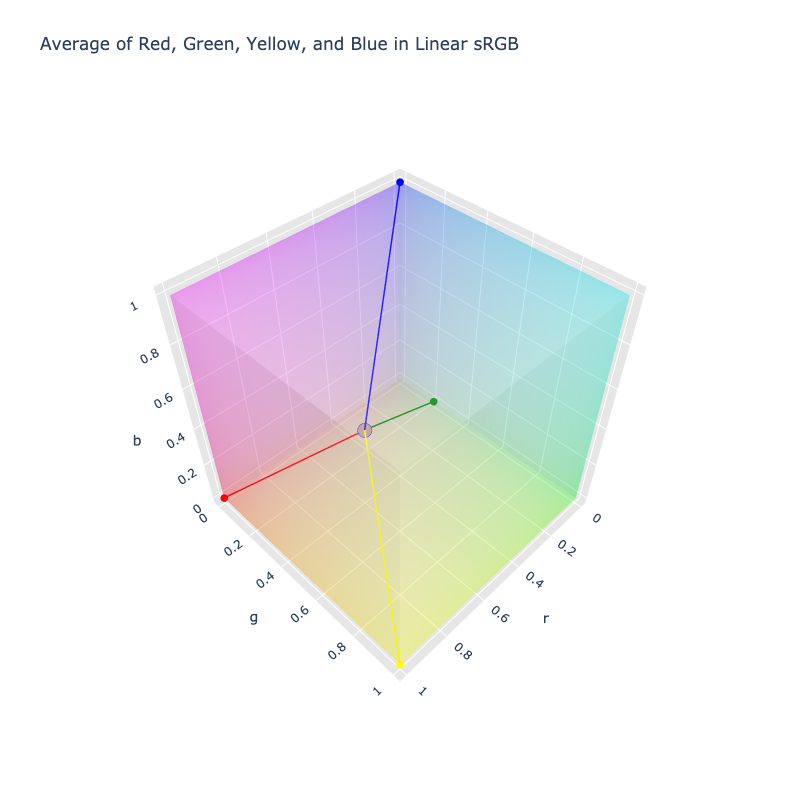
Rectangular space averaging results will often be comparable to just using weighted_mix, but there are some
differences; when performed in a polar spaces, the hue will be returned as the circular mean. Averaging this way will
always return the same results regardless of ordering.
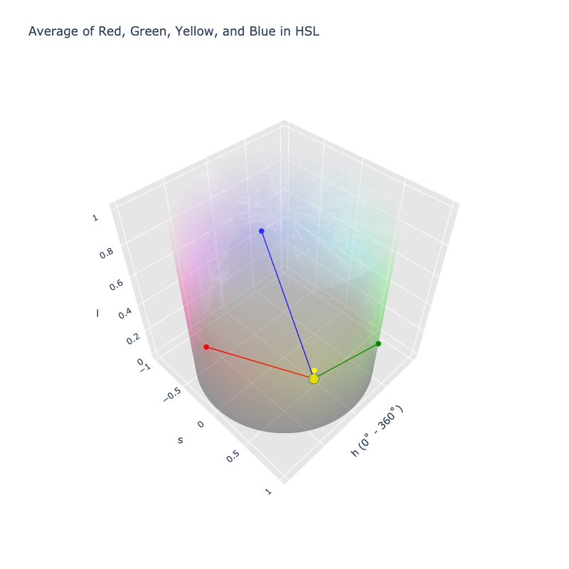
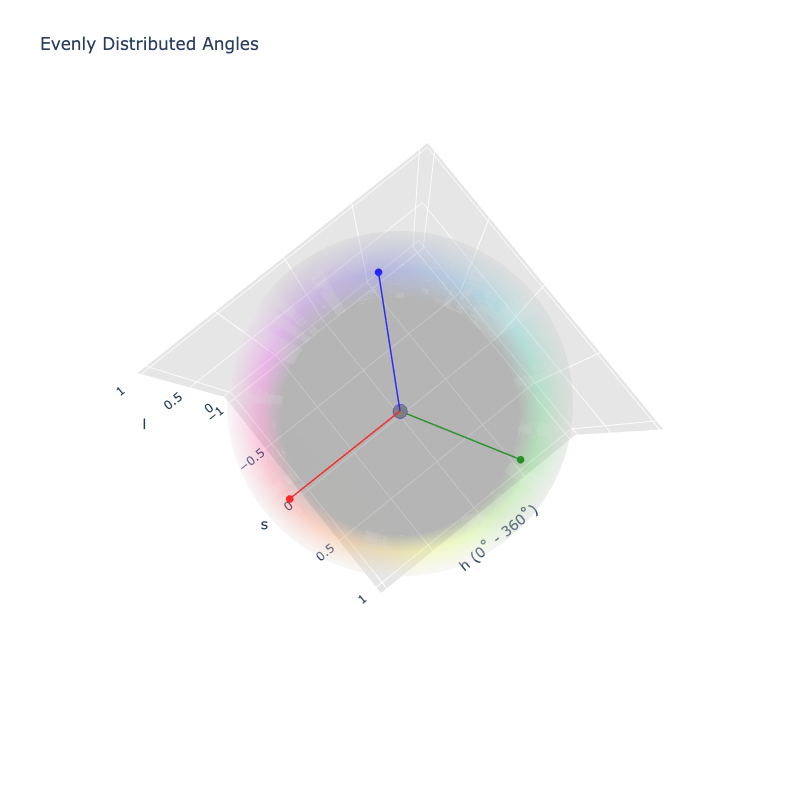
It should be noted that when averaging colors with hues which are evenly distributed around the color space, the result will produce an achromatic hue. When achromatic hues are produced during circular mean, the color will discard chroma/saturation information, producing an achromatic color.
When averaging with transparency, results will be similar to weighted_mix if using premultiplication (the default).
If premultiplication is disabled, averaging will specifically ignore colors with full transparency as such colors
provide no meaningful information to an average. This differs from how weighted_mix behaves.
>>> Steps(
...     [
...         Color.average(
...             [f'color(srgb 0 1 0 / {i / 11})', 'color(srgb 0 0 1)'],
...             premultiplied=False, space='srgb-linear'
...         )
...         for i in range(12)
...     ]
... )
[color(srgb-linear 0 0 1 / 0.5), color(srgb-linear 0 0.5 0.5 / 0.54545), color(srgb-linear 0 0.5 0.5 / 0.59091), color(srgb-linear 0 0.5 0.5 / 0.63636), color(srgb-linear 0 0.5 0.5 / 0.68182), color(srgb-linear 0 0.5 0.5 / 0.72727), color(srgb-linear 0 0.5 0.5 / 0.77273), color(srgb-linear 0 0.5 0.5 / 0.81818), color(srgb-linear 0 0.5 0.5 / 0.86364), color(srgb-linear 0 0.5 0.5 / 0.90909), color(srgb-linear 0 0.5 0.5 / 0.95455), color(srgb-linear 0 0.5 0.5 / 1)]
>>> Steps(
...     [
...         Color.weighted_mix(
...             [f'color(srgb 0 1 0 / {i / 11})', 'color(srgb 0 0 1)'],
...             premultiplied=False, space='srgb-linear'
...         )
...         for i in range(12)
...     ]
... )
[color(srgb-linear 0 0.5 0.5 / 0.5), color(srgb-linear 0 0.5 0.5 / 0.54545), color(srgb-linear 0 0.5 0.5 / 0.59091), color(srgb-linear 0 0.5 0.5 / 0.63636), color(srgb-linear 0 0.5 0.5 / 0.68182), color(srgb-linear 0 0.5 0.5 / 0.72727), color(srgb-linear 0 0.5 0.5 / 0.77273), color(srgb-linear 0 0.5 0.5 / 0.81818), color(srgb-linear 0 0.5 0.5 / 0.86364), color(srgb-linear 0 0.5 0.5 / 0.90909), color(srgb-linear 0 0.5 0.5 / 0.95455), color(srgb-linear 0 0.5 0.5 / 1)]
Lastly, powerless logic is always applied when averaging. This also differs from weighted_miz and
means that implied achromatic colors are treated as such. This is to prevent powerless hues from distorting the color
average.
Steps
Interpolation Options
Any options not consumed by mix will be passed to the underlying interpolation function. This includes options
like hue, progress, etc.
The steps method provides an intuitive interface to create lists of discrete colors. Like mixing, it is also built on
interpolate. Just provide two or more colors, and specify how many steps are wanted.
>>> Color.steps(["red", "blue"], steps=10)
[color(--oklab 0.62796 0.22486 0.12585 / 1), color(--oklab 0.60841 0.19627 0.07725 / 1), color(--oklab 0.58886 0.16768 0.02865 / 1), color(--oklab 0.56931 0.13909 -0.01995 / 1), color(--oklab 0.54976 0.1105 -0.06854 / 1), color(--oklab 0.53021 0.08191 -0.11714 / 1), color(--oklab 0.51066 0.05332 -0.16574 / 1), color(--oklab 0.49111 0.02473 -0.21433 / 1), color(--oklab 0.47156 -0.00387 -0.26293 / 1), color(--oklab 0.45201 -0.03246 -0.31153 / 1)]
If desired, multiple colors can be provided, and steps will be returned for all the interpolated segments. When interpolating multiple colors, piecewise interpolation is used (which is covered in more detail later).
>>> Color.steps(["red", "orange", "yellow", "green"], steps=10)
[color(--oklab 0.62796 0.22486 0.12585 / 1), color(--oklab 0.68287 0.16878 0.13769 / 1), color(--oklab 0.73778 0.1127 0.14954 / 1), color(--oklab 0.79269 0.05661 0.16138 / 1), color(--oklab 0.85112 0.01395 0.17378 / 1), color(--oklab 0.90955 -0.02871 0.18617 / 1), color(--oklab 0.96798 -0.07137 0.19857 / 1), color(--oklab 0.81857 -0.09435 0.16827 / 1), color(--oklab 0.66916 -0.11732 0.13797 / 1), color(--oklab 0.51975 -0.1403 0.10768 / 1)]
Steps can also be configured to return colors based on a maximum Delta E distance. This means you can ensure the distance between all colors is no greater than a certain value.
In this example, we specify the color color(display-p3 0 1 0) and interpolate steps between red.
The result gives us an array of colors, where the distance between any two colors should be no greater than the Delta E
result of 10.
>>> Color.steps(
...     [Color("display-p3", [0, 1, 0]), "red"],
...     space="lch",
...     out_space="srgb",
...     max_delta_e=10
... )
[color(srgb -0.5116 1.0183 -0.31067 / 1), color(srgb -0.4504 0.99903 -0.32673 / 1), color(srgb -0.37655 0.97943 -0.33694 / 1), color(srgb -0.27847 0.95946 -0.34286 / 1), color(srgb -0.09291 0.9391 -0.34554 / 1), color(srgb 0.23528 0.91833 -0.34574 / 1), color(srgb 0.34809 0.89715 -0.34401 / 1), color(srgb 0.42823 0.87552 -0.34098 / 1), color(srgb 0.49308 0.85343 -0.33745 / 1), color(srgb 0.54849 0.83088 -0.33349 / 1), color(srgb 0.59727 0.80784 -0.32909 / 1), color(srgb 0.64097 0.7843 -0.32423 / 1), color(srgb 0.6806 0.76025 -0.3189 / 1), color(srgb 0.71679 0.73568 -0.3131 / 1), color(srgb 0.74999 0.71057 -0.30681 / 1), color(srgb 0.78053 0.6849 -0.30002 / 1), color(srgb 0.80865 0.65865 -0.29271 / 1), color(srgb 0.83451 0.6318 -0.28486 / 1), color(srgb 0.85826 0.60433 -0.27644 / 1), color(srgb 0.87999 0.57619 -0.26744 / 1), color(srgb 0.89978 0.54736 -0.25782 / 1), color(srgb 0.9177 0.51777 -0.24752 / 1), color(srgb 0.9338 0.48735 -0.2365 / 1), color(srgb 0.9481 0.456 -0.22467 / 1), color(srgb 0.96064 0.4236 -0.21195 / 1), color(srgb 0.97145 0.38994 -0.19821 / 1), color(srgb 0.98055 0.35476 -0.18326 / 1), color(srgb 0.98796 0.31761 -0.16684 / 1), color(srgb 0.99369 0.27779 -0.14854 / 1), color(srgb 0.99777 0.23405 -0.12767 / 1), color(srgb 1.0002 0.18378 -0.10158 / 1), color(srgb 1.0009 0.11978 -0.06417 / 1), color(srgb 1 0 0 / 1)]
max_steps can be used to limit the results of max_delta_e in case result balloons to an unexpected size. Obviously,
this affects the Delta E between the colors inversely. It should be noted that steps are injected equally between every
color when satisfying a max Delta E limit in order to avoid shifting the midpoint. In some cases, in order to satisfy
both the max_delta_e and the max_steps requirement, the number of steps may even be clipped such that they are less
than the max_steps limit. max_steps is set to 1000 by default, but can be set to None if no limit is
desired.
>>> Color.steps(
...     [Color("display-p3", [0, 1, 0]), "red"],
...     space="lch",
...     out_space="srgb",
...     max_delta_e=10,
...     max_steps=10
... )
[color(srgb -0.5116 1.0183 -0.31067 / 1), color(srgb -0.09291 0.9391 -0.34554 / 1), color(srgb 0.49308 0.85343 -0.33745 / 1), color(srgb 0.6806 0.76025 -0.3189 / 1), color(srgb 0.80865 0.65865 -0.29271 / 1), color(srgb 0.89978 0.54736 -0.25782 / 1), color(srgb 0.96064 0.4236 -0.21195 / 1), color(srgb 0.99369 0.27779 -0.14854 / 1), color(srgb 1 0 0 / 1)]
When specifying a max_delta_e, steps will function as a minimum required steps and will push the delta even smaller
if the required steps is greater than the calculated steps via the maximum Delta E limit.
>>> Color.steps(
...     [Color("display-p3", [0, 1, 0]), "red"],
...     space="lch",
...     out_space="srgb",
...     max_delta_e=10,
...     steps=50
... )
[color(srgb -0.5116 1.0183 -0.31067 / 1), color(srgb -0.47276 1.0057 -0.32192 / 1), color(srgb -0.42946 0.99307 -0.33039 / 1), color(srgb -0.37992 0.98024 -0.33661 / 1), color(srgb -0.32082 0.96725 -0.341 / 1), color(srgb -0.24447 0.9541 -0.34385 / 1), color(srgb -0.1198 0.94078 -0.34542 / 1), color(srgb 0.15996 0.92729 -0.34592 / 1), color(srgb 0.26558 0.91362 -0.3455 / 1), color(srgb 0.33665 0.89976 -0.34431 / 1), color(srgb 0.3931 0.88572 -0.34248 / 1), color(srgb 0.44104 0.8715 -0.34036 / 1), color(srgb 0.48324 0.85707 -0.33806 / 1), color(srgb 0.52118 0.84244 -0.33557 / 1), color(srgb 0.55582 0.82761 -0.33289 / 1), color(srgb 0.58776 0.81258 -0.33002 / 1), color(srgb 0.61745 0.79733 -0.32696 / 1), color(srgb 0.64519 0.78187 -0.32371 / 1), color(srgb 0.67123 0.76619 -0.32025 / 1), color(srgb 0.69575 0.75029 -0.31659 / 1), color(srgb 0.7189 0.73416 -0.31273 / 1), color(srgb 0.74079 0.7178 -0.30866 / 1), color(srgb 0.76151 0.7012 -0.30437 / 1), color(srgb 0.78113 0.68437 -0.29987 / 1), color(srgb 0.79972 0.66729 -0.29515 / 1), color(srgb 0.81733 0.64995 -0.2902 / 1), color(srgb 0.834 0.63236 -0.28502 / 1), color(srgb 0.84977 0.6145 -0.2796 / 1), color(srgb 0.86467 0.59636 -0.27393 / 1), color(srgb 0.87872 0.57794 -0.26801 / 1), color(srgb 0.89194 0.55922 -0.26182 / 1), color(srgb 0.90434 0.54018 -0.25536 / 1), color(srgb 0.91596 0.52082 -0.2486 / 1), color(srgb 0.92679 0.50111 -0.24154 / 1), color(srgb 0.93686 0.48103 -0.23415 / 1), color(srgb 0.94616 0.46054 -0.22641 / 1), color(srgb 0.95471 0.43961 -0.2183 / 1), color(srgb 0.96252 0.41819 -0.20979 / 1), color(srgb 0.96959 0.39623 -0.20082 / 1), color(srgb 0.97593 0.37364 -0.19136 / 1), color(srgb 0.98155 0.35032 -0.18134 / 1), color(srgb 0.98644 0.32615 -0.17067 / 1), color(srgb 0.99062 0.30093 -0.15926 / 1), color(srgb 0.99409 0.27439 -0.14694 / 1), color(srgb 0.99685 0.24615 -0.13353 / 1), color(srgb 0.99891 0.21556 -0.11841 / 1), color(srgb 1.0002 0.18152 -0.10034 / 1), color(srgb 1.0009 0.14177 -0.07755 / 1), color(srgb 1.0008 0.09013 -0.04535 / 1), color(srgb 1 0 0 / 1)]
steps uses the color class's default ∆E method to calculate max ∆E, the current default ∆E being ∆E*ab. While
using something like ∆E*00 is far more accurate, it is a much more expensive operation. If desired, the class's
default ∆E can be changed via subclassing the color object and changing DELTA_E class variable or by manually
specifying the method via the delta_e parameter.
>>> Color.steps(
...     [Color("display-p3", [0, 1, 0]), "red"],
...     space="lch",
...     out_space="srgb",
...     max_delta_e=10,
...     delta_e="76"
... )
[color(srgb -0.5116 1.0183 -0.31067 / 1), color(srgb -0.4504 0.99903 -0.32673 / 1), color(srgb -0.37655 0.97943 -0.33694 / 1), color(srgb -0.27847 0.95946 -0.34286 / 1), color(srgb -0.09291 0.9391 -0.34554 / 1), color(srgb 0.23528 0.91833 -0.34574 / 1), color(srgb 0.34809 0.89715 -0.34401 / 1), color(srgb 0.42823 0.87552 -0.34098 / 1), color(srgb 0.49308 0.85343 -0.33745 / 1), color(srgb 0.54849 0.83088 -0.33349 / 1), color(srgb 0.59727 0.80784 -0.32909 / 1), color(srgb 0.64097 0.7843 -0.32423 / 1), color(srgb 0.6806 0.76025 -0.3189 / 1), color(srgb 0.71679 0.73568 -0.3131 / 1), color(srgb 0.74999 0.71057 -0.30681 / 1), color(srgb 0.78053 0.6849 -0.30002 / 1), color(srgb 0.80865 0.65865 -0.29271 / 1), color(srgb 0.83451 0.6318 -0.28486 / 1), color(srgb 0.85826 0.60433 -0.27644 / 1), color(srgb 0.87999 0.57619 -0.26744 / 1), color(srgb 0.89978 0.54736 -0.25782 / 1), color(srgb 0.9177 0.51777 -0.24752 / 1), color(srgb 0.9338 0.48735 -0.2365 / 1), color(srgb 0.9481 0.456 -0.22467 / 1), color(srgb 0.96064 0.4236 -0.21195 / 1), color(srgb 0.97145 0.38994 -0.19821 / 1), color(srgb 0.98055 0.35476 -0.18326 / 1), color(srgb 0.98796 0.31761 -0.16684 / 1), color(srgb 0.99369 0.27779 -0.14854 / 1), color(srgb 0.99777 0.23405 -0.12767 / 1), color(srgb 1.0002 0.18378 -0.10158 / 1), color(srgb 1.0009 0.11978 -0.06417 / 1), color(srgb 1 0 0 / 1)]
>>> Color.steps(
...     [Color("display-p3", [0, 1, 0]), "red"],
...     space="lch",
...     out_space="srgb",
...     max_delta_e=10,
...     delta_e="2000"
... )
[color(srgb -0.5116 1.0183 -0.31067 / 1), color(srgb -0.37655 0.97943 -0.33694 / 1), color(srgb -0.09291 0.9391 -0.34554 / 1), color(srgb 0.34809 0.89715 -0.34401 / 1), color(srgb 0.49308 0.85343 -0.33745 / 1), color(srgb 0.59727 0.80784 -0.32909 / 1), color(srgb 0.6806 0.76025 -0.3189 / 1), color(srgb 0.74999 0.71057 -0.30681 / 1), color(srgb 0.80865 0.65865 -0.29271 / 1), color(srgb 0.85826 0.60433 -0.27644 / 1), color(srgb 0.89978 0.54736 -0.25782 / 1), color(srgb 0.9338 0.48735 -0.2365 / 1), color(srgb 0.96064 0.4236 -0.21195 / 1), color(srgb 0.98055 0.35476 -0.18326 / 1), color(srgb 0.99369 0.27779 -0.14854 / 1), color(srgb 1.0002 0.18378 -0.10158 / 1), color(srgb 1 0 0 / 1)]
And much like interpolate, we can use stops and hints and any
of the other supported interpolate features as well.
>>> Color.steps(['orange', stop('purple', 0.25), 'green'], method='bspline', steps=10)
[color(--oklab 0.77622 0.10745 0.12653 / 1), color(--oklab 0.63152 0.10732 0.04549 / 1), color(--oklab 0.51729 0.10441 -0.01706 / 1), color(--oklab 0.4869 0.08248 -0.02304 / 1), color(--oklab 0.47734 0.05796 -0.01604 / 1), color(--oklab 0.47331 0.02733 -0.00286 / 1), color(--oklab 0.47209 -0.0077 0.01412 / 1), color(--oklab 0.47091 -0.04544 0.03249 / 1), color(--oklab 0.46706 -0.0842 0.04987 / 1), color(--oklab 0.45779 -0.12229 0.06387 / 1)]
Masking
If desired, we can mask off specific channels that we do not wish to interpolate. Masking works by cloning the color
and setting the specified channels as undefined (internally set to NaN). When interpolating, if one color's channel
has a NaN, the other color's channel will be used as the result, keeping that channel at a constant value. If both
colors have a NaN for the same channel, then NaN will be returned.
Magic Behind NaN
There are times when NaN values can happen naturally, such as with achromatic colors with hues. To learn more,
check out Undefined Handling/NaN Handling.
In the following example, we have a base color of lch(52% 58.1 22.7) which we then interpolate with
lch(56% 49.1 257.1). We then mask off the second color's channels except for hue. Applying this logic, we
will end up with a range of colors that maintains the same lightness and chroma as the first color, but with different
hues. We can see as we step through the colors that only the hue is interpolated.
>>> i = Color.interpolate(
...     ["lch(52% 58.1 22.7)", Color("lch(56% 49.1 257.1)").mask(['lightness', 'chroma', 'alpha'])],
...     space="lch"
... )
>>> [i(x/10).to_string() for x in range(10)]
['lch(52 58.1 22.7)', 'lch(52 58.1 10.14)', 'lch(52 58.1 357.58)', 'lch(52 58.1 345.02)', 'lch(52 58.1 332.46)', 'lch(52 58.1 319.9)', 'lch(52 58.1 307.34)', 'lch(52 58.1 294.78)', 'lch(52 58.1 282.22)', 'lch(52 58.1 269.66)']
You can also create inverted masks. An inverted mask will mask all except the specified channel.
>>> i = Color.interpolate(
...     ["lch(52% 58.1 22.7)", Color("lch(56% 49.1 257.1)").mask('hue', invert=True)],
...     space="lch"
... )
>>> [i(x/10).to_string() for x in range(10)]
['lch(52 58.1 22.7)', 'lch(52 58.1 10.14)', 'lch(52 58.1 357.58)', 'lch(52 58.1 345.02)', 'lch(52 58.1 332.46)', 'lch(52 58.1 319.9)', 'lch(52 58.1 307.34)', 'lch(52 58.1 294.78)', 'lch(52 58.1 282.22)', 'lch(52 58.1 269.66)']
Easing Functions
When interpolating, whether using linear interpolation or something like B-Spline interpolation, the transitioning
between colors is always linear in time, even if the path to those colors is not. For example, if you are interpolating
between 2 colors and you request a 0.5 point on that line, it will always be in the middle. This is because, no
matter how crooked the path, the rate of change on that path is always linear.
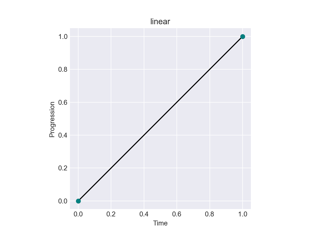
By default, ColorAide uses linear transitions when interpolating, but there are times that a different, more dynamic
transition may be desired. This can be achieved by using the progress parameter on any of the interpolation related
functions provided by ColorAide.
progress accepts an easing function that takes a single time input and returns a new time input. This allows for a
user to augment the rate of change when transitioning from one color to another. Inputs are almost always between 0 - 1
unless extrapolate is enabled and the user has manually input a range beyond 0 - 1. Even a change in
domain will not affect the range as once the domain is accounted for, internally the domain [0, 1] is used.
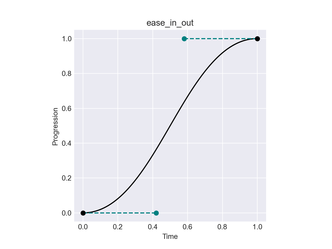
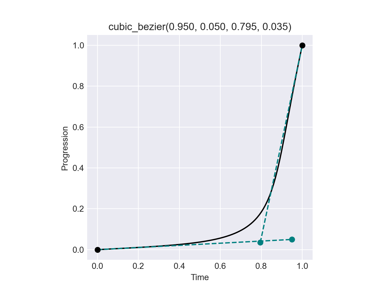
ColorAide provides 5 basic easing functions out of the box along with cubic_bezier which is used to create all of the
aforementioned easing function except linear, which simply returns what is given as an input.
Create Your Own Cubic Bezier Easings Online: https://cubic-bezier.com
| More Common Cubic Bezier Easings
The following were all acquired from https://matthewlein.com/tools/ceaser.js.
ease_in_quad = cubic_bezier(0.550, 0.085, 0.680, 0.530)
ease_in_cubic = cubic_bezier(0.550, 0.055, 0.675, 0.190)
ease_in_quart = cubic_bezier(0.895, 0.030, 0.685, 0.220)
ease_in_quint = cubic_bezier(0.755, 0.050, 0.855, 0.060)
ease_in_sine = cubic_bezier(0.470, 0.000, 0.745, 0.715)
ease_in_expo = cubic_bezier(0.950, 0.050, 0.795, 0.035)
ease_in_circ = cubic_bezier(0.600, 0.040, 0.980, 0.335)
ease_in_back = cubic_bezier(0.600, -0.280, 0.735, 0.045)

ease_out_quad = cubic_bezier(0.250, 0.460, 0.450, 0.940)
ease_out_cubic = cubic_bezier(0.215, 0.610, 0.355, 1.000)
ease_out_quart = cubic_bezier(0.165, 0.840, 0.440, 1.000)
ease_out_quint = cubic_bezier(0.230, 1.000, 0.320, 1.000)
ease_out_sine = cubic_bezier(0.390, 0.575, 0.565, 1.000)
ease_out_expo = cubic_bezier(0.190, 1.000, 0.220, 1.000)
ease_out_circ = cubic_bezier(0.075, 0.820, 0.165, 1.000)
ease_out_back = cubic_bezier(0.175, 0.885, 0.320, 1.275)

ease_in_out_quad = cubic_bezier(0.455, 0.030, 0.515, 0.955)
ease_in_out_cubic = cubic_bezier(0.645, 0.045, 0.355, 1.000)
ease_in_out_quart = cubic_bezier(0.770, 0.000, 0.175, 1.000)
ease_in_out_quint = cubic_bezier(0.860, 0.000, 0.070, 1.000)
ease_in_out_sine = cubic_bezier(0.445, 0.050, 0.550, 0.950)
ease_in_out_expo = cubic_bezier(1.000, 0.000, 0.000, 1.000)
ease_in_out_circ = cubic_bezier(0.785, 0.135, 0.150, 0.860)
ease_in_out_back = cubic_bezier(0.680, -0.550, 0.265, 1.550)
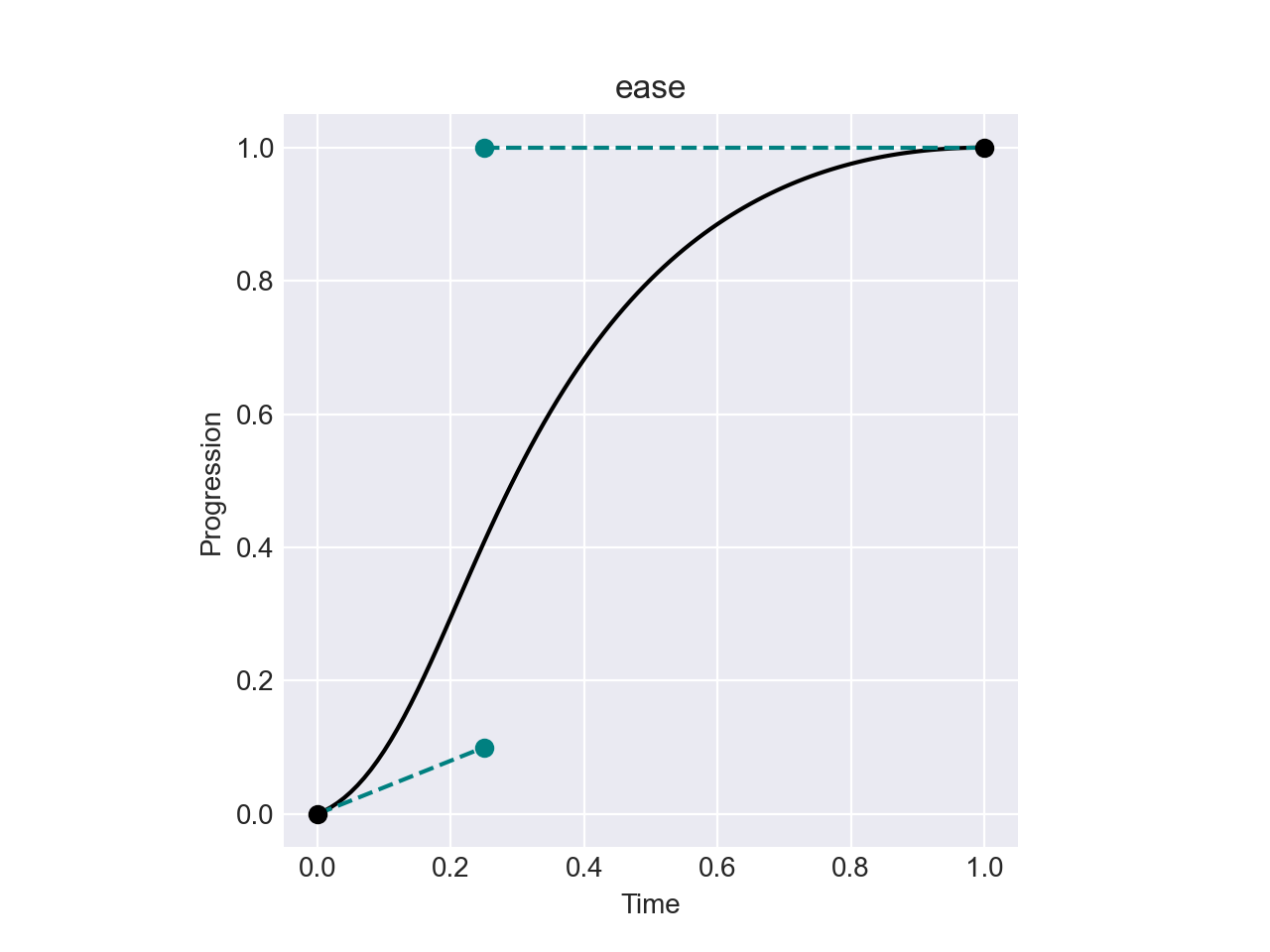
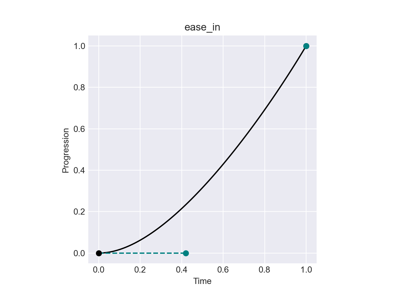
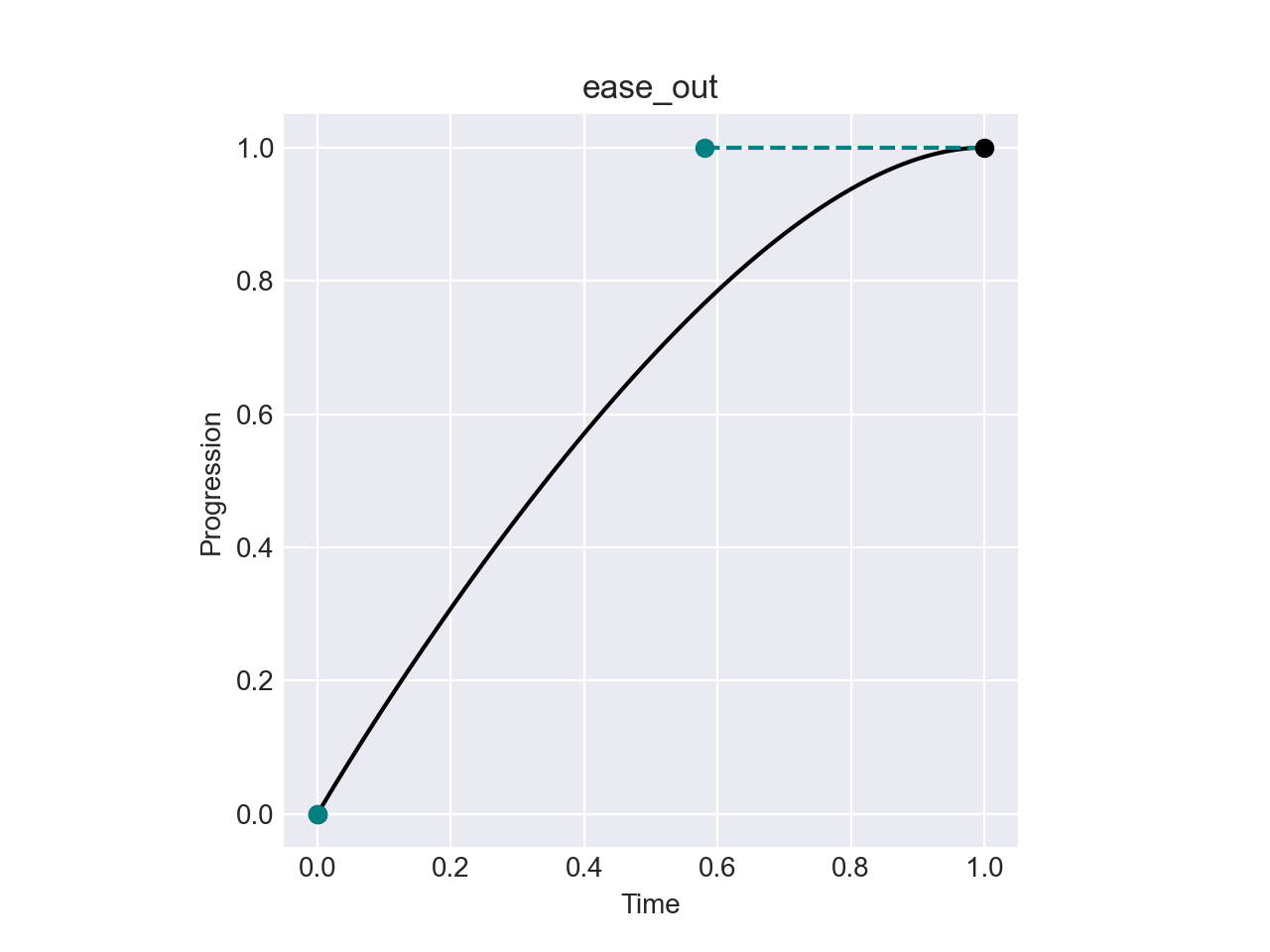
Here, we are using the default "ease in" and "ease out" easing functions provided by ColorAide.
>>> from coloraide import ease_in, ease_out
>>> Color.interpolate(
...     ["green", "blue"],
...     progress=ease_in
... )
<coloraide.interpolate.linear.InterpolatorLinear object at 0x7fc17c771450>
>>> Color.interpolate(
...     ["green", "blue"]
... )
<coloraide.interpolate.linear.InterpolatorLinear object at 0x7fc17c771e50>
>>> Color.interpolate(
...     ["green", "blue"],
...     progress=ease_out
... )
<coloraide.interpolate.linear.InterpolatorLinear object at 0x7fc17c771450>
Additionally, easing functions can be injected inline which allows a user to control how easing is performed between specific sub-interpolations within piecewise interpolation.
ColorAide even lets you apply easing functions to specific channels, though they can only be done this way for the
entire operation. This can be done to one or more channels at a time. Below, we apply an exponential "ease in" to
alpha while allowing all other channels to interpolate normally.
We can also set all the channels to an easing function via all and then override specific channels. In this case,
we exponentially "ease out" on all channels except the red channel, which we then force to be linear.
Color Stops and Hints
Color stops are the position where the transition to and from a color starts and ends. By default, color stops are evenly distributed within the domain of [0, 1], but if desired, these color stops can be shifted.
To specify color stops, simply wrap a color in a coloraide.stop object and specify the stop position. Stop positions
will then cause the transition of the targeted color to be moved.
Color stops follow the rules as laid out in the CSS spec.
CSS gradients also have a concept of "hints". Hints essentially define the midpoint between two colors. Instead of reinventing the wheel, and further complicating the interface, we've decided to just demonstrate color hints with easing functions. The logic comes directly from the CSS spec.
Using the hint function, we can generate a midpoint easing method that moves the middle of the interpolation
transition to the specified point which is relative to the two color stops it is between.
Padding
Particularly when interpolating a color scale, it can be useful to "resize" the area of the color scale being evaluated.
This can generally be done using the padding parameter. Consider the following example using the ColorBrewer scale
OrRd.
>>> scale = ['#fff7ec', '#fee8c8', '#fdd49e', '#fdbb84', '#fc8d59', '#ef6548', '#d7301f', '#b30000', '#7f0000']
>>> Color.interpolate(scale, space='srgb')
<coloraide.interpolate.linear.InterpolatorLinear object at 0x7fc17c771c50>
>>> Color.discrete(scale, space='srgb', steps=5)
<coloraide.interpolate.linear.InterpolatorLinear object at 0x7fc17c771d50>
>>> Color.interpolate(scale, space='srgb', padding=0.25)
<coloraide.interpolate.linear.InterpolatorLinear object at 0x7fc17c771c50>
>>> Color.discrete(scale, space='srgb', steps=5, padding=0.25)
<coloraide.interpolate.linear.InterpolatorLinear object at 0x7fc17c771450>
Padding can be applied to both sides by specifying a single number, or it can be controlled per side by sending in a sequence of two values.
Negative padding is allowed as well.
If the result extends past the limits, extrapolate needs to be enabled or the values will be clamped
to the ends.
>>> scale = ['#fff7ec', '#fee8c8', '#fdd49e', '#fdbb84', '#fc8d59', '#ef6548', '#d7301f', '#b30000', '#7f0000']
>>> Color.discrete(scale, space='srgb', steps=5, padding=[1, 1])
<coloraide.interpolate.linear.InterpolatorLinear object at 0x7fc17c771c50>
>>> Color.discrete(scale, space='srgb', steps=5, padding=[1, 1], extrapolate=True)
<coloraide.interpolate.linear.InterpolatorLinear object at 0x7fc17c771450>
Domains
By default, interpolation has an input domain of [0, 1]. This domain applies to an entire interpolation, even ones that span multiple colors. Generally, this is sufficient and can be used to generate color scales, mixes, and steps in any way that a user needs. When generating colors that should align with data, custom domains can be quite helpful.
For instance, associating colors with temperature.
>>> i = Color.interpolate(
...     ['blue', 'green', 'yellow', 'orange', 'red'],
...     domain=[-32, 32, 60, 85, 95]
... )
>>> i(-32)
color(--oklab 0.45201 -0.03246 -0.31153 / 1)
>>> i(47)
color(--oklab 0.75988 -0.10337 0.15637 / 1)
>>> i(89)
color(--oklab 0.7268 0.12391 0.14717 / 1)
>>> i
<coloraide.interpolate.linear.InterpolatorLinear object at 0x7fc17c771450>
It should be noted that you are not constrained to provide the exact same amount of domain values as you have colors and can have differing amounts, but if you want to align specific colors to certain data points, then it helps.
>>> Color.interpolate(
...     ['blue', 'green', 'yellow', 'orange', 'red'],
...     domain=[-32, 32, 60, 85, 95]
... )
<coloraide.interpolate.linear.InterpolatorLinear object at 0x7fc17c771c50>
>>> Color.interpolate(
...     ['blue', 'green', 'yellow', 'orange', 'red'],
...     domain=[-32, 95]
... )
<coloraide.interpolate.linear.InterpolatorLinear object at 0x7fc17c771d50>
Domains can also be specified in descending order.
>>> Color.interpolate(
...     ['blue', 'green', 'yellow', 'orange', 'red'],
...     domain=[95, 85, 60, 32, -32]
... )
<coloraide.interpolate.linear.InterpolatorLinear object at 0x7fc17c771c50>
>>> Color.interpolate(
...     ['blue', 'green', 'yellow', 'orange', 'red'],
...     domain=[95, -32]
... )
<coloraide.interpolate.linear.InterpolatorLinear object at 0x7fc17c771450>
Lastly, while domains can be specified in either ascending or descending order, it needs to be consistent. If a values increase in values, and suddenly decreases in value, you will get discontinuities.
>>> i = Color.interpolate(
...     ['blue', 'green', 'yellow', 'orange', 'red'],
...     domain=[-32, 32, 60, 20, 95]
... )
>>> i.domain
<bound method Interpolator.domain of <coloraide.interpolate.linear.InterpolatorLinear object at 0x7fc17c771450>>
>>> i
<coloraide.interpolate.linear.InterpolatorLinear object at 0x7fc17c771450>
Custom domains are most useful when working with discrete or
interpolate directly, but you can use it in other methods like steps as well. As
steps does not take data point inputs like interpolate, we do not need to use the temperature data as an input
except to set the domain, but the steps will be generated with the same alignment relative to the domain range.
>>> Color.interpolate(
...     ['blue', 'green', 'yellow', 'orange', 'red'],
...     domain=[-32, 32, 60, 85, 95]
... )
<coloraide.interpolate.linear.InterpolatorLinear object at 0x7fc17c771c50>
>>> Color.discrete(
...     ['blue', 'green', 'yellow', 'orange', 'red'],
...     domain=[-32, 32, 60, 85, 95]
... )
<coloraide.interpolate.linear.InterpolatorLinear object at 0x7fc17c771e50>
>>> Color.steps(
...     ['blue', 'green', 'yellow', 'orange', 'red'],
...     steps=11,
...     domain=[-32, 32, 60, 85, 95]
... )
[color(--oklab 0.45201 -0.03246 -0.31153 / 1), color(--oklab 0.46546 -0.05386 -0.22834 / 1), color(--oklab 0.4789 -0.07526 -0.14516 / 1), color(--oklab 0.49234 -0.09666 -0.06197 / 1), color(--oklab 0.50578 -0.11806 0.02122 / 1), color(--oklab 0.51922 -0.13946 0.1044 / 1), color(--oklab 0.71505 -0.11027 0.14728 / 1), color(--oklab 0.91836 -0.079 0.18851 / 1), color(--oklab 0.90067 -0.02222 0.18429 / 1), color(--oklab 0.81162 0.04279 0.1654 / 1), color(--oklab 0.62796 0.22486 0.12585 / 1)]
Wile you can technically feed domain into mix, it is probably not as useful. It will respect the domain
alignment, but mix always accepts a percentage of [0, 1], regardless of the underlying domain.
Extrapolation
By default, ColorAide clamps the entire progress of an interpolation to always be within the domain ([0, 1] by default). In most cases, this is more what most user expects and why this is the default. It should be noted that this does not affect easing functions, as the clamping is done prior to any easing function calls.
If it is desired to extrapolate past 0 and 1, extrapolate can set to True on all interpolation methods.
As a larger example, we can purposely interpolate over a range with values beyond 0 and 1. Here we extended the range to -0.5 and 1.5.
>>> offset, factor = 0.25, 1.5
>>> i = Color.interpolate(['red', 'blue'], space='srgb')
>>> Ramp([i((r * factor / 100) - offset) for r in range(101)])
[color(srgb 1 0 0 / 1), color(srgb 1 0 0 / 1), color(srgb 1 0 0 / 1), color(srgb 1 0 0 / 1), color(srgb 1 0 0 / 1), color(srgb 1 0 0 / 1), color(srgb 1 0 0 / 1), color(srgb 1 0 0 / 1), color(srgb 1 0 0 / 1), color(srgb 1 0 0 / 1), color(srgb 1 0 0 / 1), color(srgb 1 0 0 / 1), color(srgb 1 0 0 / 1), color(srgb 1 0 0 / 1), color(srgb 1 0 0 / 1), color(srgb 1 0 0 / 1), color(srgb 1 0 0 / 1), color(srgb 0.995 0 0.005 / 1), color(srgb 0.98 0 0.02 / 1), color(srgb 0.965 0 0.035 / 1), color(srgb 0.95 0 0.05 / 1), color(srgb 0.935 0 0.065 / 1), color(srgb 0.92 0 0.08 / 1), color(srgb 0.905 0 0.095 / 1), color(srgb 0.89 0 0.11 / 1), color(srgb 0.875 0 0.125 / 1), color(srgb 0.86 0 0.14 / 1), color(srgb 0.845 0 0.155 / 1), color(srgb 0.83 0 0.17 / 1), color(srgb 0.815 0 0.185 / 1), color(srgb 0.8 0 0.2 / 1), color(srgb 0.785 0 0.215 / 1), color(srgb 0.77 0 0.23 / 1), color(srgb 0.755 0 0.245 / 1), color(srgb 0.74 0 0.26 / 1), color(srgb 0.725 0 0.275 / 1), color(srgb 0.71 0 0.29 / 1), color(srgb 0.695 0 0.305 / 1), color(srgb 0.68 0 0.32 / 1), color(srgb 0.665 0 0.335 / 1), color(srgb 0.65 0 0.35 / 1), color(srgb 0.635 0 0.365 / 1), color(srgb 0.62 0 0.38 / 1), color(srgb 0.605 0 0.395 / 1), color(srgb 0.59 0 0.41 / 1), color(srgb 0.575 0 0.425 / 1), color(srgb 0.56 0 0.44 / 1), color(srgb 0.545 0 0.455 / 1), color(srgb 0.53 0 0.47 / 1), color(srgb 0.515 0 0.485 / 1), color(srgb 0.5 0 0.5 / 1), color(srgb 0.485 0 0.515 / 1), color(srgb 0.47 0 0.53 / 1), color(srgb 0.455 0 0.545 / 1), color(srgb 0.44 0 0.56 / 1), color(srgb 0.425 0 0.575 / 1), color(srgb 0.41 0 0.59 / 1), color(srgb 0.395 0 0.605 / 1), color(srgb 0.38 0 0.62 / 1), color(srgb 0.365 0 0.635 / 1), color(srgb 0.35 0 0.65 / 1), color(srgb 0.335 0 0.665 / 1), color(srgb 0.32 0 0.68 / 1), color(srgb 0.305 0 0.695 / 1), color(srgb 0.29 0 0.71 / 1), color(srgb 0.275 0 0.725 / 1), color(srgb 0.26 0 0.74 / 1), color(srgb 0.245 0 0.755 / 1), color(srgb 0.23 0 0.77 / 1), color(srgb 0.215 0 0.785 / 1), color(srgb 0.2 0 0.8 / 1), color(srgb 0.185 0 0.815 / 1), color(srgb 0.17 0 0.83 / 1), color(srgb 0.155 0 0.845 / 1), color(srgb 0.14 0 0.86 / 1), color(srgb 0.125 0 0.875 / 1), color(srgb 0.11 0 0.89 / 1), color(srgb 0.095 0 0.905 / 1), color(srgb 0.08 0 0.92 / 1), color(srgb 0.065 0 0.935 / 1), color(srgb 0.05 0 0.95 / 1), color(srgb 0.035 0 0.965 / 1), color(srgb 0.02 0 0.98 / 1), color(srgb 0.005 0 0.995 / 1), color(srgb 0 0 1 / 1), color(srgb 0 0 1 / 1), color(srgb 0 0 1 / 1), color(srgb 0 0 1 / 1), color(srgb 0 0 1 / 1), color(srgb 0 0 1 / 1), color(srgb 0 0 1 / 1), color(srgb 0 0 1 / 1), color(srgb 0 0 1 / 1), color(srgb 0 0 1 / 1), color(srgb 0 0 1 / 1), color(srgb 0 0 1 / 1), color(srgb 0 0 1 / 1), color(srgb 0 0 1 / 1), color(srgb 0 0 1 / 1), color(srgb 0 0 1 / 1), color(srgb 0 0 1 / 1)]
>>> i = Color.interpolate(['red', 'blue'], space='srgb', extrapolate=True)
>>> Ramp([i((r * factor / 100) - offset) for r in range(101)])
[color(srgb 1.25 0 -0.25 / 1), color(srgb 1.235 0 -0.235 / 1), color(srgb 1.22 0 -0.22 / 1), color(srgb 1.205 0 -0.205 / 1), color(srgb 1.19 0 -0.19 / 1), color(srgb 1.175 0 -0.175 / 1), color(srgb 1.16 0 -0.16 / 1), color(srgb 1.145 0 -0.145 / 1), color(srgb 1.13 0 -0.13 / 1), color(srgb 1.115 0 -0.115 / 1), color(srgb 1.1 0 -0.1 / 1), color(srgb 1.085 0 -0.085 / 1), color(srgb 1.07 0 -0.07 / 1), color(srgb 1.055 0 -0.055 / 1), color(srgb 1.04 0 -0.04 / 1), color(srgb 1.025 0 -0.025 / 1), color(srgb 1.01 0 -0.01 / 1), color(srgb 0.995 0 0.005 / 1), color(srgb 0.98 0 0.02 / 1), color(srgb 0.965 0 0.035 / 1), color(srgb 0.95 0 0.05 / 1), color(srgb 0.935 0 0.065 / 1), color(srgb 0.92 0 0.08 / 1), color(srgb 0.905 0 0.095 / 1), color(srgb 0.89 0 0.11 / 1), color(srgb 0.875 0 0.125 / 1), color(srgb 0.86 0 0.14 / 1), color(srgb 0.845 0 0.155 / 1), color(srgb 0.83 0 0.17 / 1), color(srgb 0.815 0 0.185 / 1), color(srgb 0.8 0 0.2 / 1), color(srgb 0.785 0 0.215 / 1), color(srgb 0.77 0 0.23 / 1), color(srgb 0.755 0 0.245 / 1), color(srgb 0.74 0 0.26 / 1), color(srgb 0.725 0 0.275 / 1), color(srgb 0.71 0 0.29 / 1), color(srgb 0.695 0 0.305 / 1), color(srgb 0.68 0 0.32 / 1), color(srgb 0.665 0 0.335 / 1), color(srgb 0.65 0 0.35 / 1), color(srgb 0.635 0 0.365 / 1), color(srgb 0.62 0 0.38 / 1), color(srgb 0.605 0 0.395 / 1), color(srgb 0.59 0 0.41 / 1), color(srgb 0.575 0 0.425 / 1), color(srgb 0.56 0 0.44 / 1), color(srgb 0.545 0 0.455 / 1), color(srgb 0.53 0 0.47 / 1), color(srgb 0.515 0 0.485 / 1), color(srgb 0.5 0 0.5 / 1), color(srgb 0.485 0 0.515 / 1), color(srgb 0.47 0 0.53 / 1), color(srgb 0.455 0 0.545 / 1), color(srgb 0.44 0 0.56 / 1), color(srgb 0.425 0 0.575 / 1), color(srgb 0.41 0 0.59 / 1), color(srgb 0.395 0 0.605 / 1), color(srgb 0.38 0 0.62 / 1), color(srgb 0.365 0 0.635 / 1), color(srgb 0.35 0 0.65 / 1), color(srgb 0.335 0 0.665 / 1), color(srgb 0.32 0 0.68 / 1), color(srgb 0.305 0 0.695 / 1), color(srgb 0.29 0 0.71 / 1), color(srgb 0.275 0 0.725 / 1), color(srgb 0.26 0 0.74 / 1), color(srgb 0.245 0 0.755 / 1), color(srgb 0.23 0 0.77 / 1), color(srgb 0.215 0 0.785 / 1), color(srgb 0.2 0 0.8 / 1), color(srgb 0.185 0 0.815 / 1), color(srgb 0.17 0 0.83 / 1), color(srgb 0.155 0 0.845 / 1), color(srgb 0.14 0 0.86 / 1), color(srgb 0.125 0 0.875 / 1), color(srgb 0.11 0 0.89 / 1), color(srgb 0.095 0 0.905 / 1), color(srgb 0.08 0 0.92 / 1), color(srgb 0.065 0 0.935 / 1), color(srgb 0.05 0 0.95 / 1), color(srgb 0.035 0 0.965 / 1), color(srgb 0.02 0 0.98 / 1), color(srgb 0.005 0 0.995 / 1), color(srgb -0.01 0 1.01 / 1), color(srgb -0.025 0 1.025 / 1), color(srgb -0.04 0 1.04 / 1), color(srgb -0.055 0 1.055 / 1), color(srgb -0.07 0 1.07 / 1), color(srgb -0.085 0 1.085 / 1), color(srgb -0.1 0 1.1 / 1), color(srgb -0.115 0 1.115 / 1), color(srgb -0.13 0 1.13 / 1), color(srgb -0.145 0 1.145 / 1), color(srgb -0.16 0 1.16 / 1), color(srgb -0.175 0 1.175 / 1), color(srgb -0.19 0 1.19 / 1), color(srgb -0.205 0 1.205 / 1), color(srgb -0.22 0 1.22 / 1), color(srgb -0.235 0 1.235 / 1), color(srgb -0.25 0 1.25 / 1)]
Lastly, it is important to note that this affects stops as well, mainly stops applied to interpolation endpoints. When an endpoint is moved inwards via a color stop, the end range of the interpolation is clamped, extending the start and end color. But when extrapolation is enabled, a color stop on an endpoint essentially moves the start and end interpolation. And since there are no other colors on either end to interpolate with, extrapolation occurs.
>>> Color.interpolate([stop('red', 0.25), stop('blue', 0.75)], space='srgb')
<coloraide.interpolate.linear.InterpolatorLinear object at 0x7fc17c771c50>
>>> Color.interpolate([stop('red', 0.25), stop('blue', 0.75)], space='srgb', extrapolate=True)
<coloraide.interpolate.linear.InterpolatorLinear object at 0x7fc17c771450>
Undefined/NaN Handling
Color spaces that have hue coordinates often have rules about when the hue is considered relevant. For instance, in the HSL color space, if saturation is zero, the hue is essentially powerless. This is because the color is "without color" or achromatic; therefore, the hue can have no affect on the actual color.
ColorAide will generally respect the values a user provides, so if an achromatic HSL color is given a hue of 270 degrees, ColorAide will accept it, but the hue will not affect the color in any meaningful way.
During conversions, such context is lost, and if an achromatic color is converted to the color space like HSL, the resultant color will have a hue that is noted as undefined. This is simply because there is no good hue for achromatic colors as they play no part in the color. Any hue is actually incorrect as achromatic colors have no real hue. Instead, colors will be returned with a value that represents that the hue is missing or undefined, or maybe better worded, could not be defined.
Many libraries, like d3-color, chroma.js, and
color.js, represent null hues with NaN (not a number). This is usually done
to make color interpolation easier. Some, like d3-color, are a bit more liberal with NaN and will target special cases
that are above and beyond the normal rules to help ensure good interpolation. For instance, they not only mark hue
undefined on HSL colors when saturation is zero, but they'll mark saturation as NaN when lightness indicates "black"
or "white".
ColorAide also uses NaN, or in Python float('nan'), to represent undefined channels. In certain situations,
when a hue is deemed undefined, the hue value will be set to coloraide.NaN, which is just a constant containing
float('nan').
When performing linear interpolation, where only two color's channels are ever being evaluated together at a given time,
if one color's channel has a NaN, the other color's channel will be used as the result. If both colors have a NaN
for the same channel, then NaN will be returned.
Continuous NaN Handling
NaN handling is a bit different for the Continuous and
Cubic Spline interpolation approaches. Linear only evaluates colors at a given time,
while the others will take into consideration more than two colors. Because the context is much wider and more
complicated, NaN values will often get context from both sides.
Notice that in this example, because white's saturation is zero, the hue is undefined. Because the hue is undefined,
when the color is mixed with a second color (green), the hue of the second color is used.
But if we manually set the hue to 0 instead of NaN, we can see that the mixing goes quite differently.
Technically, any channel can be set to NaN. And there are various ways to do this. The
Color Manipulation documentation goes into the details of how these NaN values
naturally occur and the various ways a user and manipulate them.
Carrying-Forward
Experimental
This feature is provided to give parity with CSS behavior. As the spec is still in flux, behavior is subject to change or feature could be removed entirely. Use at your own risk.
CSS introduces the concept of carrying-forward undefined channels of like color spaces during conversion to the interpolating color space. The idea is to provide a sane handling to users who specified undefined channels for interpolation, but did not account for the conversion to the interpolating color space.
If a color has undefined channels, and is converting to a like color space, after conversion the new color will have the same undefined channels, assuming the channels support carrying-forward. The example below demonstrates the concept.
ColorAide, by default, expects the user to be aware that undefined values are lost if conversion is required for
interpolation. This is mainly because the intent of the color can be changed during this process, but some users may
find the automatic carrying-forward more convenient. For this reason, ColorAide has implemented carrying-forward as an
optional feature via the carryforward option.
In this example, interpolating without carrying-forward results in an interpolation between a purplish color and white. Using carrying-forward, we get a purplish color with an undefined green channel. The green channel takes on the white's green channel giving us an interpolation between a more greenish color and white.
>>> Color.interpolate(['color(srgb 0.5 none 0.8)', 'white'], space='display-p3')
<coloraide.interpolate.linear.InterpolatorLinear object at 0x7fc17c771450>
>>> Color.interpolate(['color(srgb 0.5 none 0.8)', 'white'], space='display-p3', carryforward=True)
<coloraide.interpolate.linear.InterpolatorLinear object at 0x7fc17c771c50>
Depending on the color space, carrying-forward may have better or worse results.
The following table shows channel components supported for carryforward. Spaces may use different names for their
channels, but if they are derived from the related space classes, their channels are supported. For instance, xyz is
derived from RGBish, so x, y, and z is treated like super saturated r, g, and b.
| Space Type | Channel Equivalents |
|---|---|
RGBish |
r, g, b |
Labish |
l |
LChish |
l, c, h |
HSLish |
h, s, l |
HSVish |
h, s, v |
Cylindrical |
h |
Carrying-forward is applied within categories.
| Category | Components |
|---|---|
| Reds | r |
| Greens | g |
| Blues | b |
| Lightness | l |
| Colorfulness | c, s |
| Hue | h |
| Opponent a | a |
| Opponent b | b |
| Value | v |
Additionally, carryforward is applied to analogous sets as well. This means that a combination of components are
considered equivalent to another set of components. For instance, if an LChish space has an undefined chroma and hue,
when converting to a Labish space, a and b would be considered undefined (and vice versa). If all color components
are undefined, then when converted, all components in the new space would also be undefined.
Powerless Hues
Experimental
This feature is provided to give parity with CSS behavior. As the spec is still in flux, behavior is subject to change or feature could be removed entirely. Use at your own risk.
Normally, ColorAide respects the user's explicitly defined hues. This gives the user power to do things like masking off all channels but the hue in order to interpolate only the hue channel.
But when doing this, a user must explicitly define the hue as achromatic if they want the hue to be ignored. Conversions of achromatic colors to a cylindrical space will, in most cases, have the hue automatically set to undefined.
>>> Color.interpolate(['oklch(1 0 0)', 'oklch(0.75 0.2 180)'], space='oklch')
<coloraide.interpolate.linear.InterpolatorLinear object at 0x7fc17c771c50>
>>> Color.interpolate(['oklch(1 0 None)', 'oklch(0.75 0.2 180)'], space='oklch')
<coloraide.interpolate.linear.InterpolatorLinear object at 0x7fc17c771e50>
CSS has the concept of powerless hues which causes explicitly defined hues to be powerless (or act as
undefined) when a color is considered achromatic. This means a user never has to think about
achromatic hues, so even if they erroneously define a hue, the hue will automatically be treated as undefined when
interpolating. ColorAide implements this behavior via the powerless option.
>>> Color.interpolate(
...     ['oklch(1 0 0)', 'oklch(0.75 0.2 180)'],
...     space='oklch',
...     powerless=True
... )
<coloraide.interpolate.linear.InterpolatorLinear object at 0x7fc17c771d50>
>>> Color.interpolate(
...     ['oklch(1 0 None)', 'oklch(0.75 0.2 180)'],
...     space='oklch',
...     powerless=True
... )
<coloraide.interpolate.linear.InterpolatorLinear object at 0x7fc17c771450>
The one downside is that control over the hue will be diminished to some degree as ColorAide will no longer respect a user's explicit hue if the color is determined to be achromatic.
>>> Color.interpolate(
...     ['oklch(none none 0)', 'oklch(0.75 0.2 360)'],
...     space='oklch',
...     hue='specified'
... )
<coloraide.interpolate.linear.InterpolatorLinear object at 0x7fc17c771450>
>>> Color.interpolate(
...     ['oklch(none none 0)', 'oklch(0.75 0.2 360)'],
...     space='oklch',
...     hue='specified',
...     powerless=True
... )
<coloraide.interpolate.linear.InterpolatorLinear object at 0x7fc17c771f50>